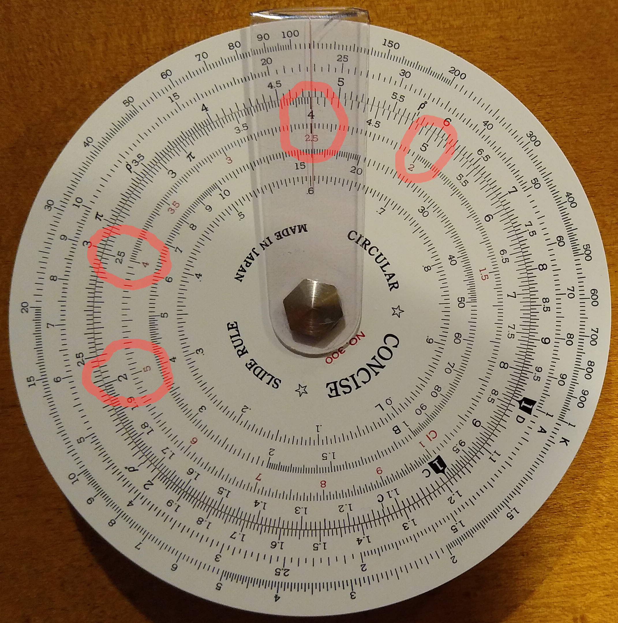
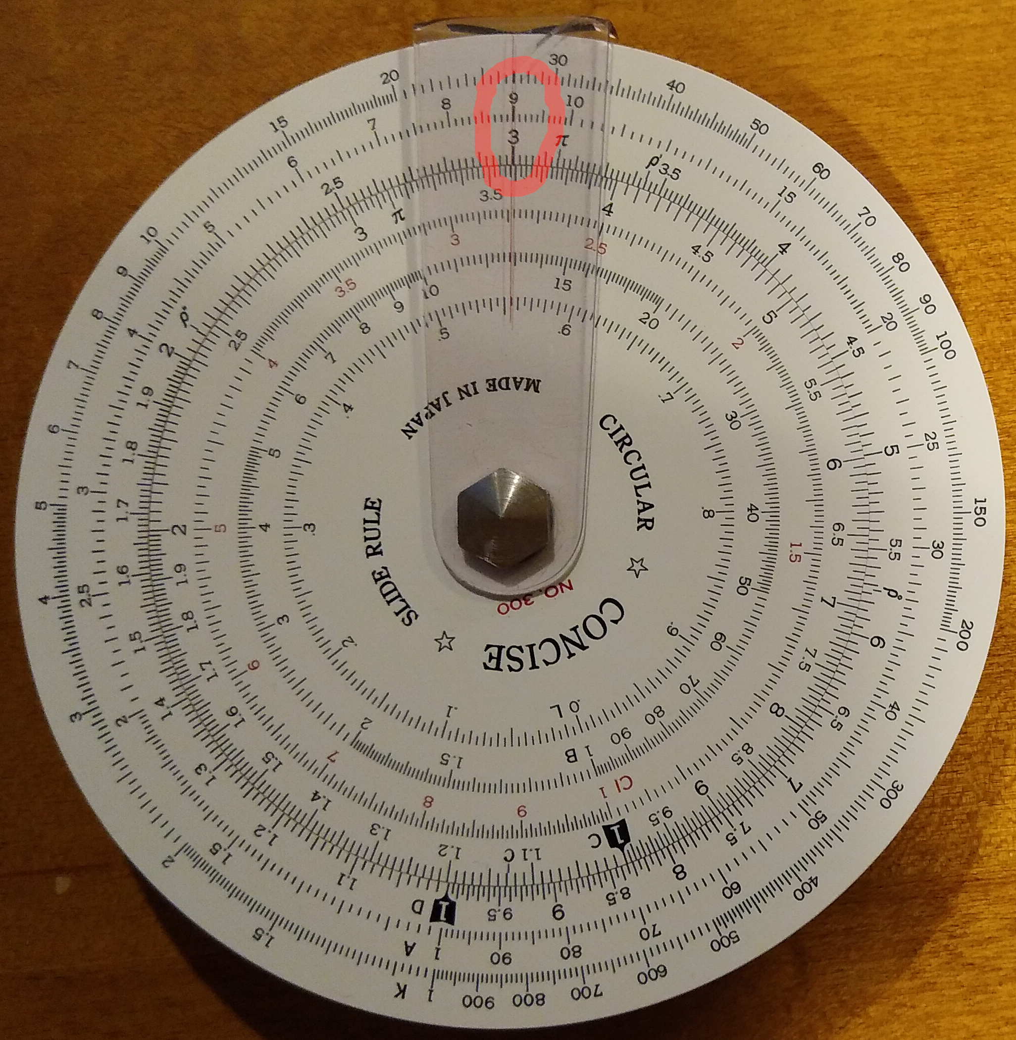
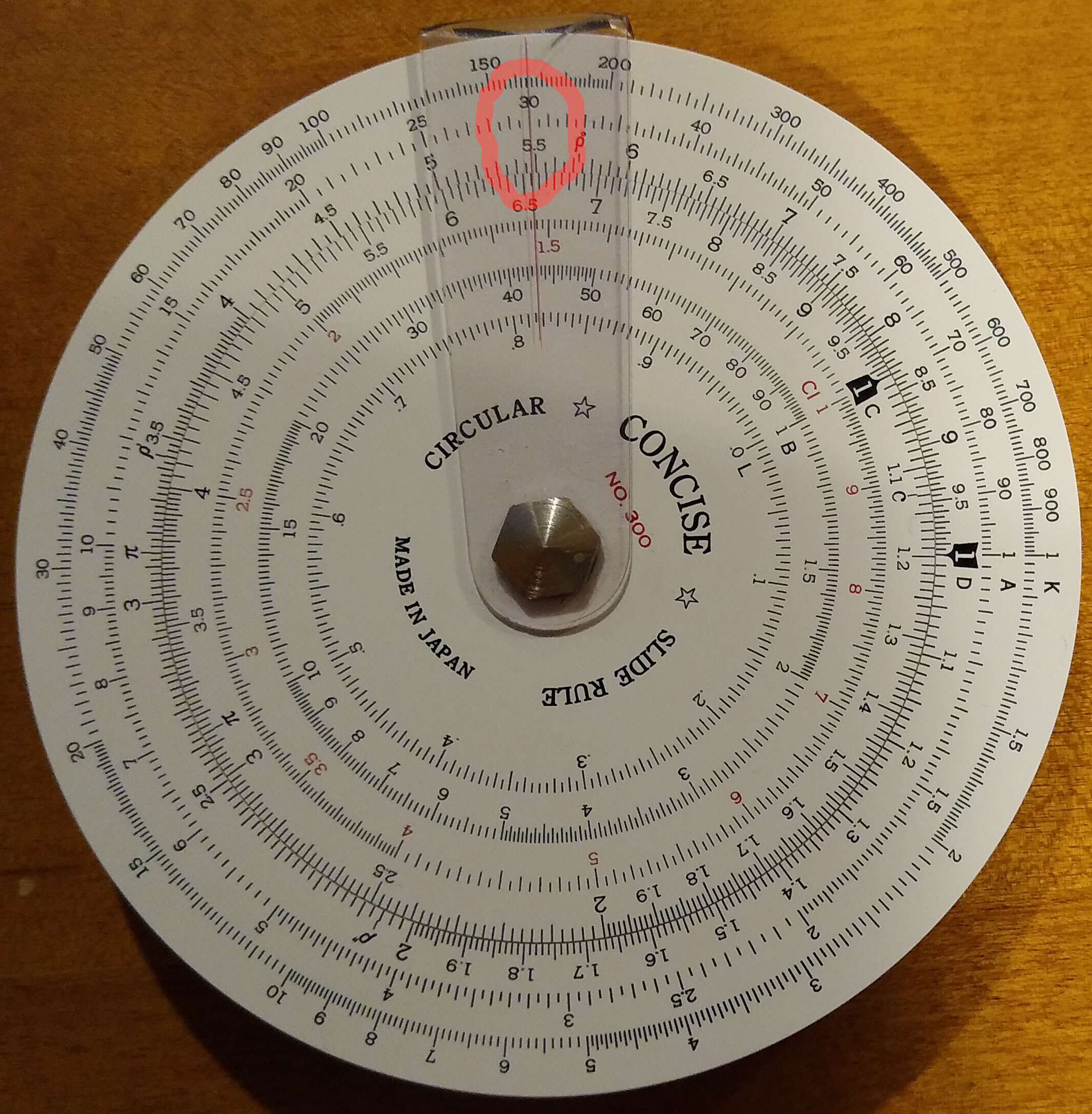
Category Archives: Math

Audio Phase: Shift versus Inversion

It is said that a 180* phase shift is the same as a polarity inversion. That is, it flips a wave to its mirror-image across the time axis. If we imagine a simple sin or cos wave, we see that this is true. 180* is half a wavelength, slide it that distance either forward or back, and you get the same wave with polarity inverted. Another consequence of this lies in audio room tuning. If the distance between 2 walls is half a wavelength of a particular frequency, the wave reflecting from the wall, being inverted polarity, cancels the wave arriving which causes a dip or null at that frequency. Those same walls will also boost waves at twice that frequency because that same distance between the walls is their full wavelength, so the reflected wave is in phase with the arriving one.

But this doesn’t work with a general musical waveform. No amount of sliding it left (back) or right (forward) in time will invert its polarity. Intuitively, we see that a musical wave is not symmetric or repeating like a sin or cos wave. The musical waveform is much more complex, containing hundreds of frequencies all superimposed. Any distance we slide it left or right represents a phase shift at only 1 particular frequency. Alternately, sliding it left or right can be seen as a phase shift at all frequencies, but a different phase angle for each, since the distance it shifted is a different number of wavelengths for each frequency it contains. As in the above example, it boosts some frequencies and cuts others. This is what happens in a comb filter.

Since every frequency has a different wavelength, it’s hard to imagine how a phase shift of the same angle at all frequencies could even be possible. It is possible, but to do it we need to expand into another dimension and use complex numbers. That computation creates a new waveform that is the polarity inverted version of the original. You can find explanations of this all over the internet, for example here: https://www.audiosciencereview.com/forum/index.php?threads/analytical-analysis-polarity-vs-phase.29331/

Because of this, when speaking of music and audio I prefer the term “polarity inversion” to “180* phase shift”. Even though they can be equivalent, the former is concise while the latter is somewhat ambiguous since one must also specify at what frequencies the phase shift is applied.

Audio: How Much Data is That?

It’s easy to compute but I figured I’d save it here for reference

RatebPSBPSKB/secMins/GBCD ratioNotes
44.1-161,411,200176,400172.271011.00Redbook CD
44.1-242,116,800264,600258.4671.50
48-161,536,000192,000187.5931.09
48-242,304,000288,000281.25621.63Standard DVD
88.2-244,233,600529,200516.80333.00
96-244,608,000576,000562.5313.27Popular for modern classical music recordings
176.4-248,467,2001,058,4001,033.616.96.00
192-249,216,0001,152,0001,125.015.56.53

This represents actual data bits to represent the music – no overhead. If you want to know what bandwidth is needed to carry an SPDIF signal at a given rate, add extra for packet overhead.

The formula is simple:

bits per second = S * C * B
S = sample rate (samples per second)
C = channels (2 for stereo)
B = bits per sample

For example for CD we have

S = 44100
C = 2
B = 16
S * C * B = 1,411,200 bits per second

Note: most DACs internally oversample before D-A conversion. They typically oversample at the highest integer multiple of the source rate that is less than their max rate. For example the Cirrus/Wolfson WM8741 has a max rate of 192k, so CD and DVD are oversampled 4x to 176.4 and 192 respectively. This happens automatically within the DAC chip. Because of this, it’s usually pointless to oversample an audio signal before feeding it to a DAC – the DAC is going to do it anyway, so why waste processing power and bandwidth doing it yourself?

Slide Rules: Trig

Introduction and basics in Part 1. Squares, Cubes and roots in Part 2. Here we cover trigonometry: sine, cosine and tangent. Not all slide rules have these scales, but when they do they are usually labeled as follows:

  • S: sine
  • T: tangent
  • ST: sine & tangent

Notes on these scales:

Trig Scales

You don’t need both sine & cosine, since they are inverse every 1/4 circle or 90 degrees. That is, for any angle A in degrees, sin(A) = cos(90-A). That’s why slide rules don’t have a cosine scale – it’s not needed.

Knowing a few key values of sine enables one to quickly estimate many problems (like crosswinds when landing an airplane) in your head. No need for a slide rule, let alone a calculator.

  • sin(0) = 0
  • sin(30) = 0.5
  • sin(45) = 0.707
  • sin(90) = 1

For small angles, sine and tangent are almost the same. Thus many slide rules have an shared ST scale for both, for small angles – typically less than about 5*. Exactly how close are sine and tangent for small angles?

  • 2 sig figs: 15* – sin & tan differ by the 2nd sig fig
    • sin(15*) = 0.259
    • tan(15*) = 0.268
  • 3 sig figs: 2* – sin & tan differ by the 3rd sig fig
    • sin(3*) = 0.0523
    • tan(3*) = 0.0524

Slide Rules!

Background

I learned to use slide rules in high school in the 1980s. My physics teacher was one of the most memorable teachers in my life, “Mr. Jordan”. He said that slide rules can be faster than a calculator, and they promote a better understanding of numbers, orders of magnitude, and significant figures. They are not as accurate as calculators, but real-world problems only need 2-3 significant figures. As such, anyone who used a slide rule instead of a calculator would get a bonus 10% on every test, and answers would be considered correct if they were within 1% of correct. I was one of the few who took him up on this offer.

He handed out small circular slide rules, saying they were easier to use than linear slide rules (which is true, since circular never goes off scale). I don’t remember exactly what model slide rule it was, but the closest I know of today is the Concise model 28N. It was either that, or something very similar.

Note: I now have a Concise model 300, which is their biggest and best. The C and D scales are 8 cm in diameter, which is a circumference of 8π which is 25.2 cm, or about 10″. This is the slide used used in the photos below.

All we needed for physics was multiplication and division, and squares & cubes. Jordan would throw problems like, “A Porsche 944 goes 0-60 in 8 seconds. If it weighs 3000 lbs. with fuel and driver, and half the engine power goes toward acceleration, how much power does the engine produce?”

Since then I’ve been a slide rule fan. I use one when flying for computing fuel burn rates, density altitude, altimeter & airspeed corrections. I also keep one around for doing random calculations that come up during the course of a day. When 2-3 sig figs of accuracy is sufficient, it’s quicker & easier than a calculator.

Slide rules are antiquated tech. So why learn to use them? It’s for these secondary benefits mentioned above. And they are fun.

Introduction

Slide rules are based on the concept of a logarithm (aka log). Every log has a base, and the log is what power you raise that base to get some other number N. Examples:

  • Log base 10 of 100 is 2, because you raise 10 to the power 2 to get 100, or 10^2 = 100
  • Log base 2 of 32 is 5, since 2^5 = 32
  • Log base 10 of 42 is 1.623 (approximately), or 10^1.623 = 42

The reason logs are useful, and how they led to the invention of slide rules, is because exponents are additive. That is: 10^5 = 10^(2+3) = 10^2 * 10^3

That means if I know the logs of 2 numbers A and B, call them La and Lb, then La + Lb is the log of the product A*B.

Note: Computer scientists take advantage of this when multiplying many tiny numbers together. Since computer floating points have finite precision, multiplying many tiny numbers leads to underflow. Instead, take each number's log and add them all up. Then at the end take the inverse log of that sum. This gives you the same product with much higher precision since it never underflows.

Now suppose I have 2 rulers with markings from 1 to 10. But instead of being spaced linear like a normal ruler, they are spaced logarithmically. If I line up 1 on the first ruler, with some number A on the second ruler, then the mark for some other number B on the first ruler will line up with the value of A*B on the second ruler.

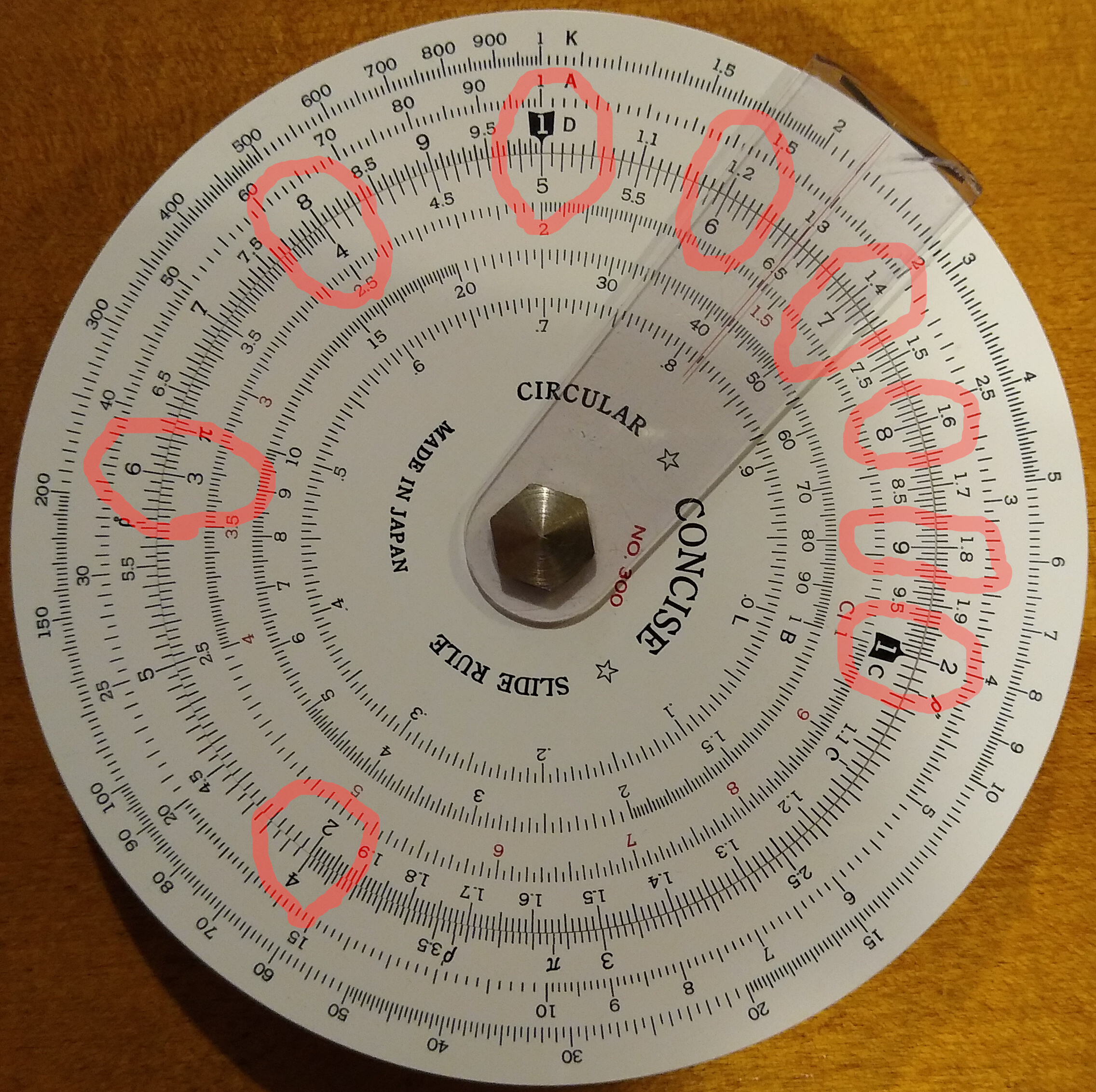
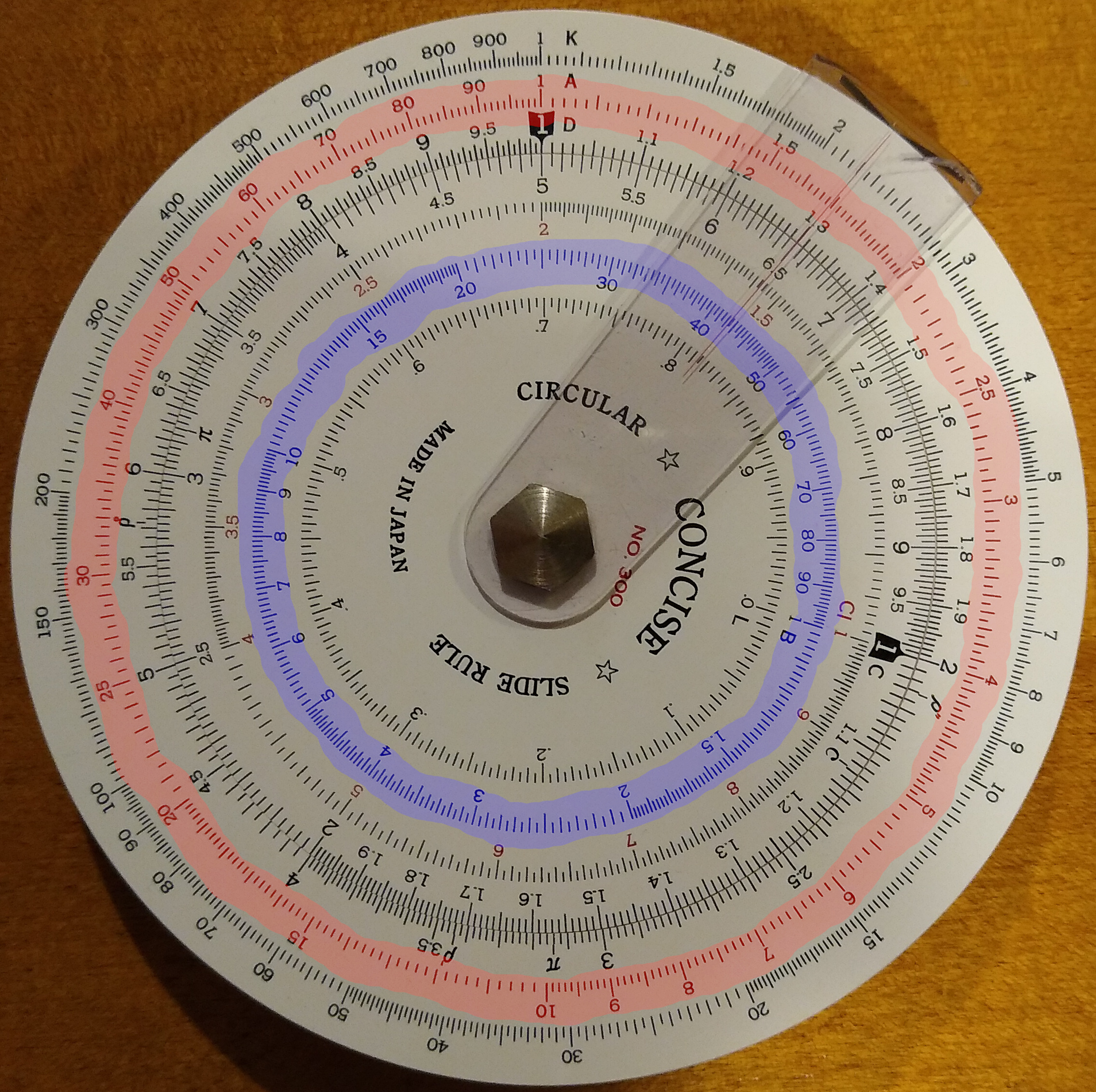
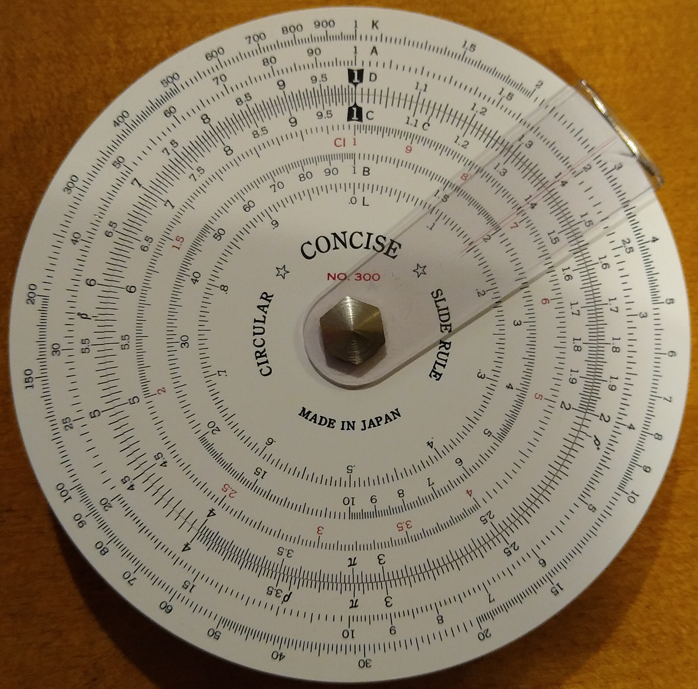
A picture’s worth 1000 words, so here’s a circular slide rule.

The clear marker with the thin red line is called the cursor. We’ll ignore that for now. See how the two black highlighted “1” values are aligned? Each of those scales (inner and outer) are logarithmic. That’s why the range from 1-2 takes about 1/3 of the scale while the range at the upper end is much more compressed. As you start from 1 and go up the scale, the numbers start out spread apart and get more squished together.

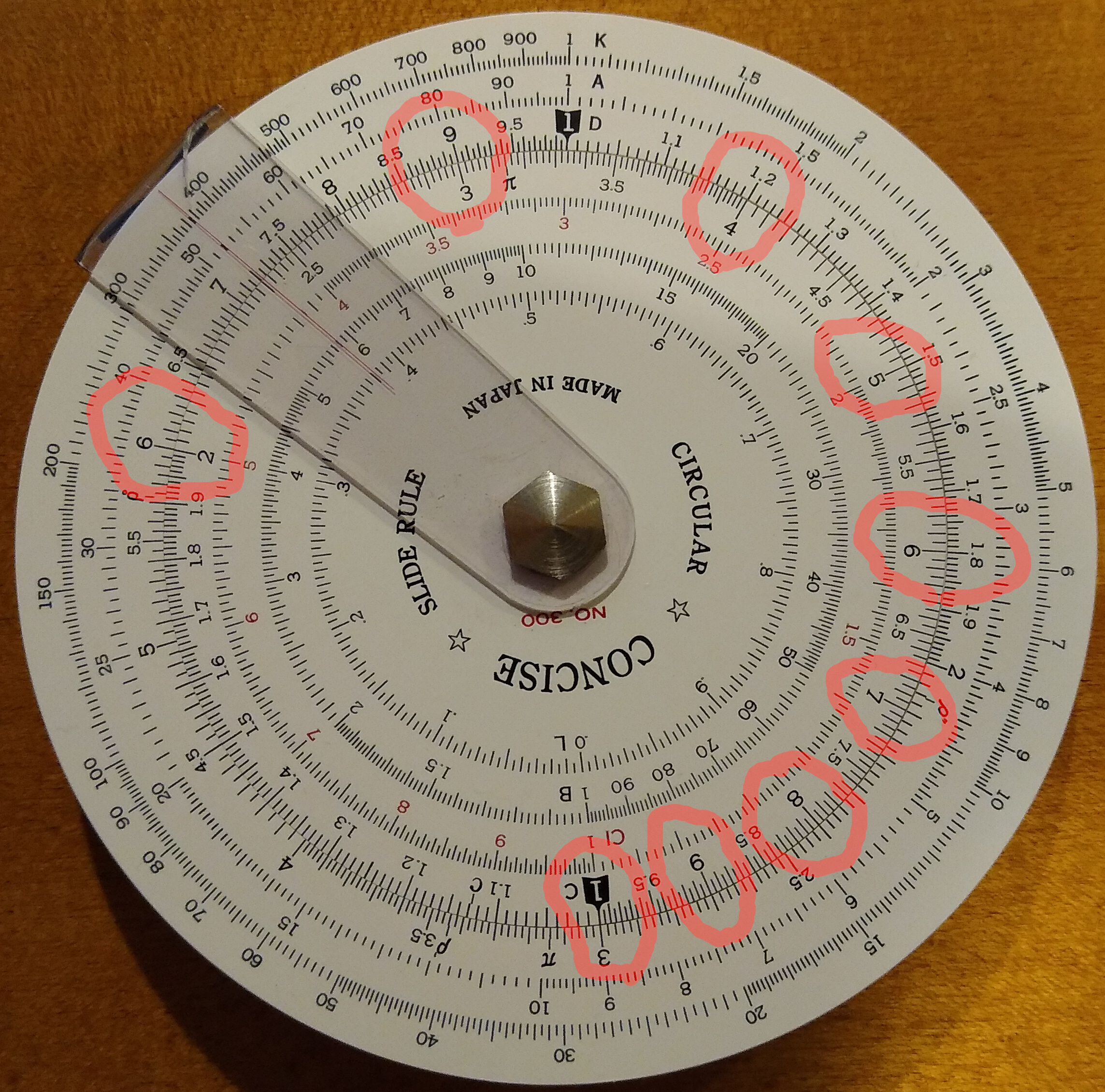
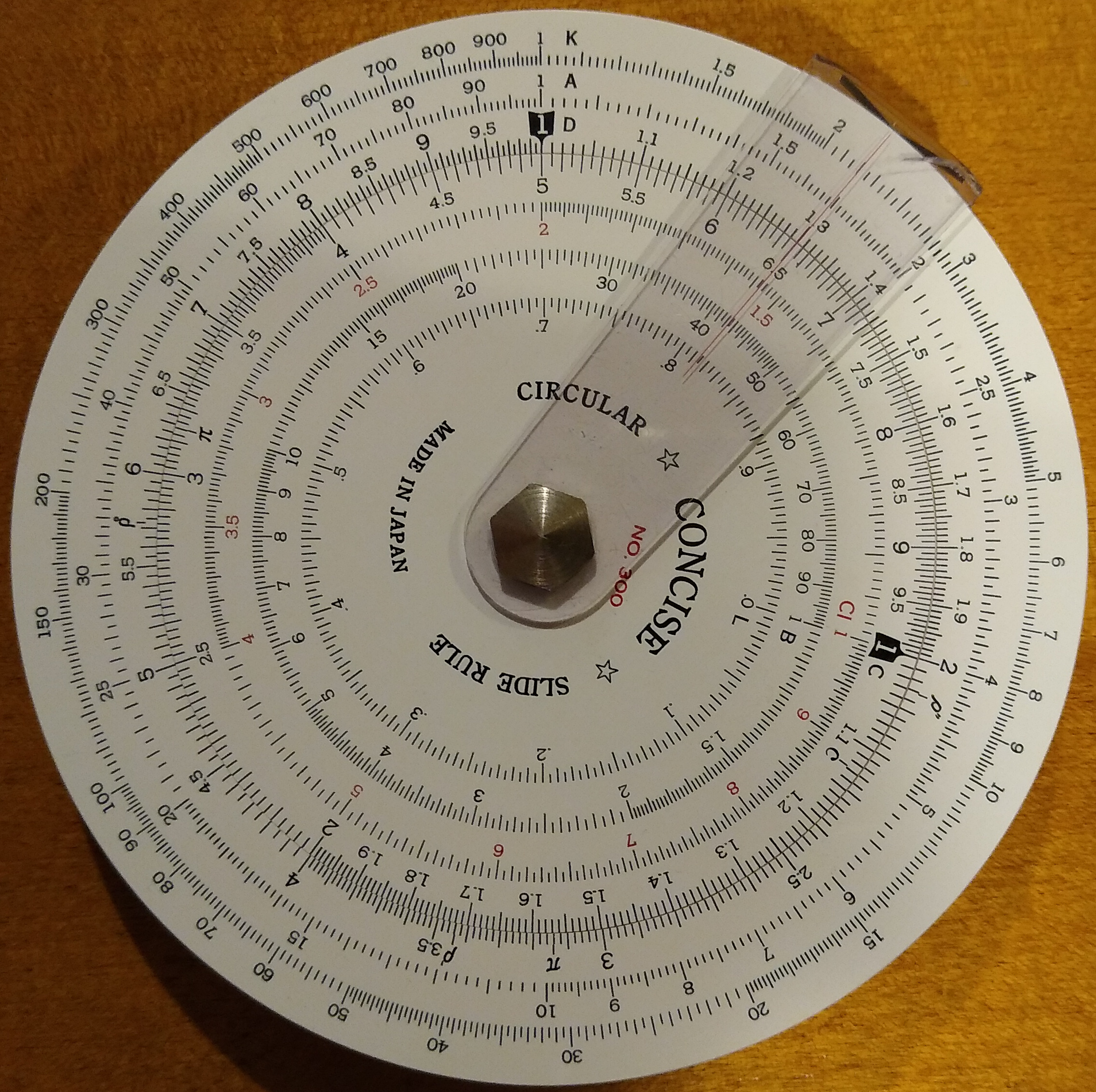
Watch what happens when we slide the inner “1” to line up with the outer “2”:

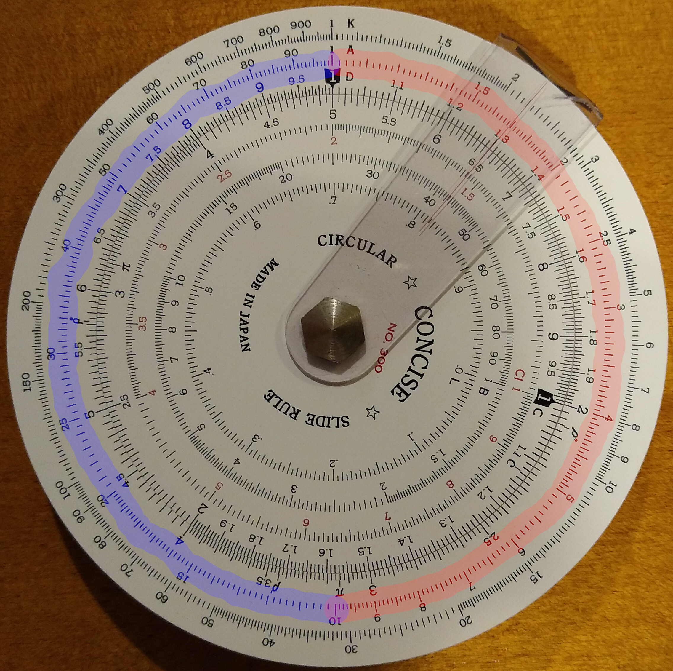
If this were a linear ruler, it would be shifted by 1 over the entire scale: 1 to 2, 2 to 3, 3 to 4, etc. But not here, where 1 matches 2, 2 matches 4, 3 matches 6, 4 matches 8, etc. Every number on the inner scale matches the number exactly twice as much on the outer scale. And every number on the outer scale matches the number exactly half as much on the inner scale.

Below I’ve highlighted what I’m talking about. Each number on the inner scale matches to exactly twice its value on the outer scale.

In short, this slide rule is set up to multiply or divide any number by 2.

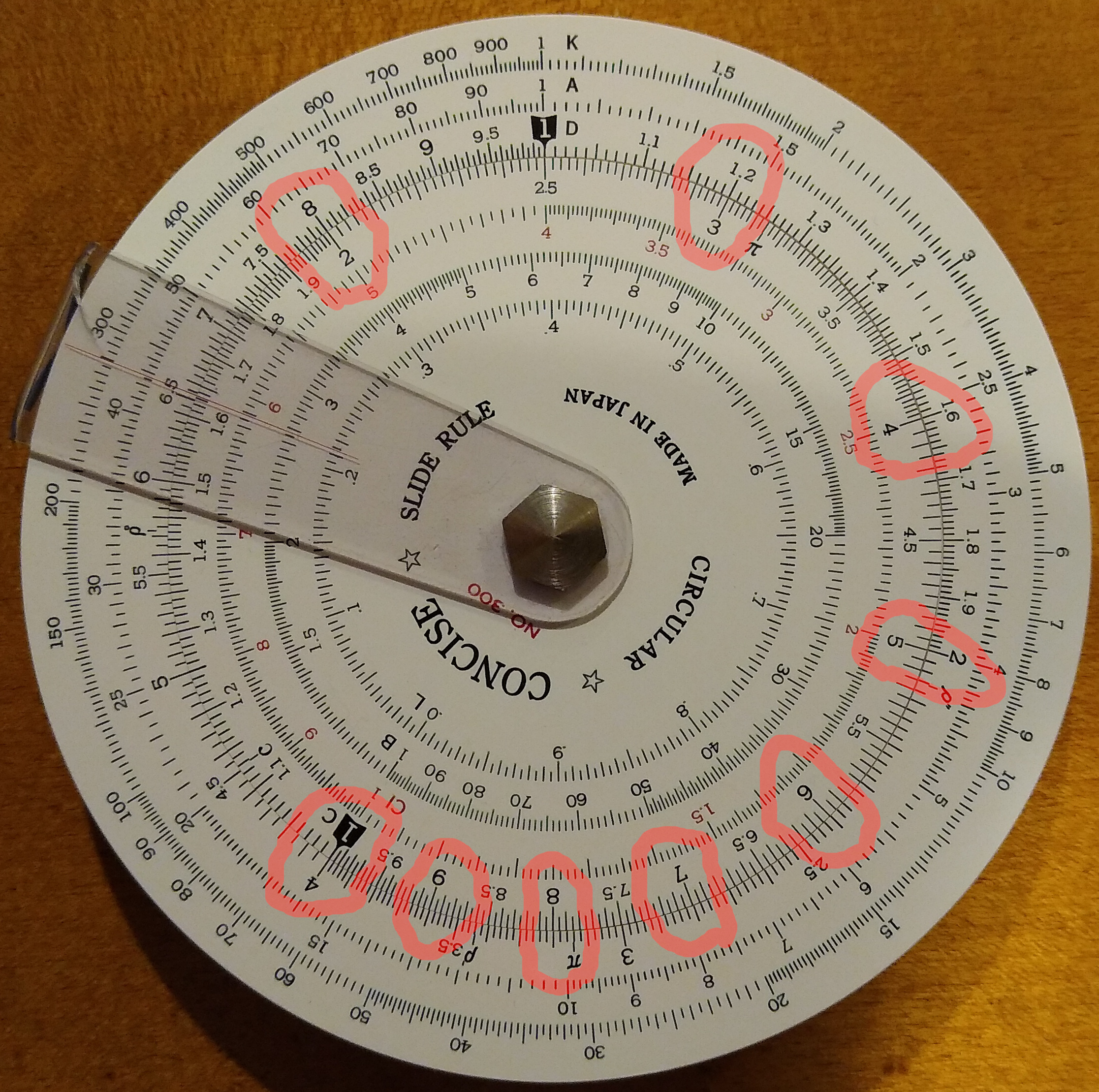
Yet here’s the kicker: this is not specific to the value 2. It’s downright magical. Here’s the slide rule with 1 matched to 3:

Similar scenario, only now we can multiply or divide any number by 3. And look below for 4:

Of course, this doesn’t just work for integers. You can do this for any number in the scale. In fact, now you know how to multiply or divide using a slide rule.

BTW, these are called the C and D scales. On this slide rule, D is the outer and C is the inner. That’s what the C and D are in photos.

What about Zeros and Decimals?

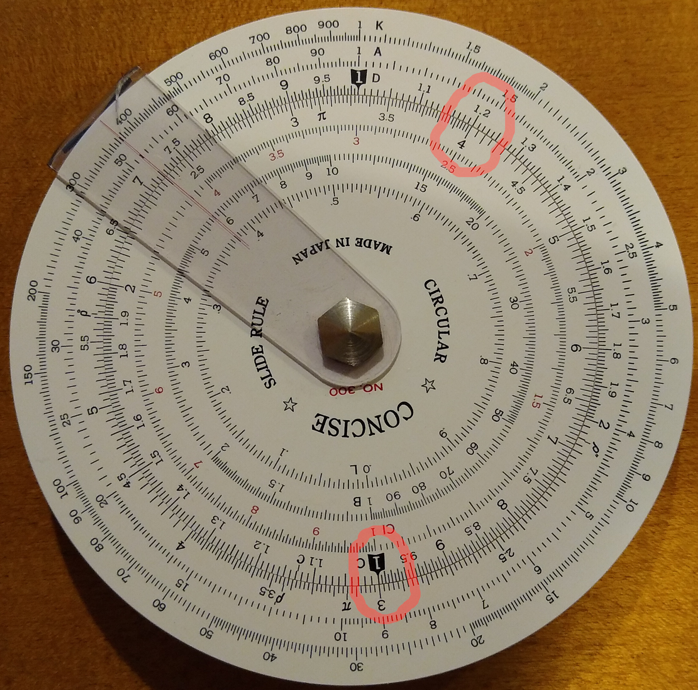
Suppose you want to multiply 3*4. First line up the C scale 1 with the D scale 3, then look at the C scale 4, which points to the D scale 12. See the picture below:

You might notice that it doesn’t actually say 12, it says 1.2. We happen to know that 3*4 is 12, so we interpret the 1.2 as 12. When you use a slide rule you need to keep track of the decimal point.

This is where circular slide rules are easier to use than straight ones. On a straight rule, this 3*4 problem is greater than 1, so it goes off scale and you can't read the answer. You need to shift to additional scales CF or DF (C folded and D folded) to read the results. Circular slide rules never go off scale, they just wrap around. Much simpler and easier!

All Those Scales!

So far we’ve only covered the C and D scales. You can see that slide rules have several other scales. Most slide rules have these scales:

  • C & D: multiplication & division
  • CI: inverses
  • A & B: squares & square roots

Some slide rules also have these scales:

  • K: cubes & cube roots
  • S, T, ST: sine & tangent

Let’s go through these one at a time.

CI Scale: Inverses

The CI scale is the inverse of the C scale and it’s marked in red. Simply put, it is the same scale but going backward – in the opposite direction. The C scale increases clockwise; the CI scale increases counter-clockwise. Each number on the C scale, lines up with its inverse on the CI scale. For example, 2 lines up with 5 since the inverse of 2 is 0.5.

Here, the cursor comes in handy to read these scales. For example, below the cursor is lined up on 4, so you can precisely read its inverse on the CI scale, which is 0.25. But as you can see all around the dial, each number on C always lines up with its inverse on CI, and both scales increase in opposite directions around the circle. I’ve marked some obvious points, like 4 and .25, 5 and .2, and their inverses.

For example, reading for yourself you can see that 1/7 is about 1.43. My calculator says it’s 1.42857. So we got 3 significant figures of accuracy there (more on sig figs later).

Conclusion

Now that you can use a slide rule for basic computations, have some fun practicing. I cover some of the other scales in part 2.

Slide Rules: Past the Basics

For background, here is part 1. It introduces slide rules and covers basic usage with C, D and CI scales. Here we cover the A, B and K scales for squares, square roots, cubes and cube roots.

A Scale: Squares and Square Roots

The A scale shows the square of each number on the D scale. Conversely, the D scale shows the square root of each number on the A scale.

Below the cursor shows that 3 on the D scale matches 9 on the A scale.

Note that as the D scale goes from 1 to 10, the A scale goes from 1 to 100. This means every single-digit number in the A scale has a corresponding double-digit number further up the scale. That is: 1 and 10, 2 and 20, 3 and 30, etc.

For example, below the cursor is on the A scale 30, showing the square root of 30 is 5.48:

So, squares are easy: just find the number on D scale and look to the corresponding number on A scale. But going the opposite direction, square roots, becomes ambiguous. What if you want the square root of a number that is not in the range of 1 to 100? For example:

  • If you want the square root of 400, on the A scale do you use 4 or 40?
  • If you want the square root of 4000,  on the A scale do you use 4 or 40?
  • If you want the square root of 0.5, on the A scale do you use 5 or 50?

First, observe that all of the single-digit numbers in the A scale occupy the first half, all the double-digit numbers the second half, and the split (the value 10) is exactly the mid-point of the scale. Thus, you can think of the A scale has having 2 halves. So the question boils down to knowing which half to use.

The answer is based on how many zeroes in the number whose root you want to know: is that number of zeroes odd or even? Adding or removing each zero (or each decimal point shift left or right) shifts back and forth between the 2 halves of the scale.

For example, consider the number 4.

  • The square root of 4 is 2 (low side of A scale).
  • The square root of 40 is 6.32 (high side of A scale).
  • The square root of 400 is 20 (low side of A scale).
  • The square root of 4000 is 63.2 (high side of A scale).

This pattern simply repeats. And it also repeats in the opposite direction:

  • The square root of 0.4 is 0.632 (high side of A scale).
  • The square root of 0.04 is 0.2 (low side of A scale).
  • The square root of 0.004 is 0.0632 (high side of A scale).

K Scale: Cubes and Cube Roots

The K scale works like the A scale. To cube any number N, find N on the D scale and look at the corresponding number on the K scale.

For example, this shows that 2 cubed is 8 (it actually shows that 2 squared is 4, and cubed is 8):

Yet the K scale also has the value 80, whose cube root is 4.31:

And the K scale also has the value 800, whose cube root is 9.28:

So while the A scale splits into 2 equal parts (1-10 and 10-100), the K scale splits into 3 equal parts: 1-10, 10-100, and 100-1000. Each of these occupies exactly 1/3 of the scale:

As with the A scale, cubing numbers is simple. Find N on the D scale and the corresponding K scale is N cubed. Yet doing the opposite, taking the cube root, is a bit more complex. You need to know which 1/3 of the scale to use. The procedure is a simple extension of what we did for the A scale. Yet since the A scale had only 2 parts, we thought of it as flipping back and forth. With the K scale having 3 parts, instead of flipping, each shift of the decimal point rotates forward to the next, or back to the prior part of the scale.

For example, consider the number 8:

  • The cube root of 8 is 2 (part 1 of  K scale).
  • The cube root of 80 is 4.31 (part 2 of K scale).
  • The cube root of 800 is 9.28 (part 3 of K scale).
  • The cube root of 8000 is 20 (part 1 of K scale).

It repeats every 3rd shift of the decimal point. And it also applies in the reverse direction as numbers get smaller:

  • The cube root of 0.8 is 0.928 (part 3 of K scale).
  • The cube root of 0.08 is 0.431 (part 2 of K scale).
  • The cube root of 0.008 is 0.2 (part 1 of K scale).

Exponents and Roots other than 2 or 3

Most everyday problems, especially those involving basic physics, use squares or cubes. Powers other than 2 or 3 are uncommon. Yet we do occasionally encounter them and you can solve them with a slide rule. The trick is to know some basic math rules about adding exponents.

Suppose we some number N, say 3.5, and we want to know N to some power, say the 7th power. So how would we compute 3.5^7 with our slide rule?

First, we split the exponent into smaller parts involving squares and cubes:

3.5^7 = 3.5^(2+2+3)

Next we split this out:

 3.5^(2+2+3) = 3.5^2 * 3.5^2 * 3.5^3

Now we have split the problem into squares and cubes so we can compute it on our slide rule:

3.5^2 = 12.2
3.5^3 = 42.8
12.2 * 12.2 * 42.8 = 150 * 42.8 = 6,430

Checking this with a calculator, I get 6,433.9. The slide rule gave us 3 significant figures.

Note: you can apply this same method with roots by taking the exponents as fractions. That is, the square root of 2 is 2 to the 1/2 power, cube root of 2 is 2 so the 1/3 power, etc.

What About that B Scale?

The B scale is the same as the A scale, used for squares and square roots. But it corresponds with the C scale instead of the D scale. Using D-A is the same as C-B. The B scale isn’t essential, but it is sometimes useful. On the Concise model 300, the A scale is along the outer circumference and the B scale is further inside. This makes the A scale longer and more accurate.

To quantify, on this Concise model 300 the A scale has a diameter of 9.2 cm and B scale 5.9. The A scale is 9.2 / 5.9 = 1.56 times longer. That’s a significant difference!

Conclusion

With squares and cubes, the power of the slide rule increases and we can solve a wider variety of problems. The next step is trigonometry: sine, cosine, tangent. These come up frequently in simple physics and everyday problems. This is covered in part 3.


Sanity Check: 0-60 Times

With electric cars, the classic performance metric of 0-60 time has gotten much faster, approaching the theoretical limits of available traction. Yet some cars show 0-60 times even faster than this, which seems impossible. Accelerating faster than available traction requires thrust that doesn’t depend on traction, like jet or rocket engines.

I suspect that the 0-60 times being quoted for some of these cars are not real, but just theoretical projections based on power to weight ratio. Here’s a way to sanity check them.

Braking is already traction limited. So when acceleration is also traction limited, the car should accelerate 0-60 in the same distance and time it takes to brake from 60-0. These might be slightly different, due to the car’s uneven front-rear weight distribution and different sized tires front and rear. But it’s still a good rough guide and sanity check.

Braking 60-0 is usually given as distance rather than time. But assuming constant acceleration (not exactly true but a decent approximation) it’s easy to convert. Remember our basic formulas:

v = a*t
d = 1/2 * a * t²

The best street legal tires have a maximum traction of about 1.1 G. You can get up to about 1.3 G with R compound racing tires, but most are not street legal and the ones that are, don’t last more than 1,000 miles.

Here’s how we compute this for 1.1 G with English units:

60 mph = 88 fps
1 G = 32 fps/s
v = a*t --> 88 = 32 * 1.1 * t --> t = 2.5 secs
d = 1/2 * a * t² --> d = 1/2 * 32 * 1.1 * 2.5² --> d = 110 feet

Braking from 60 to 0 at 1.1 G takes 2.5 seconds and 110 feet. If you look at the highest performance cars, this is about equal to their tested braking performance. So, that same car cannot accelerate 0-60 any faster than 2.5 seconds because no matter how much power it has, that is the limit of available traction.

Some cars claim to do 0-60 in 2 seconds flat. This is 1.375 G of acceleration and takes 88 feet of distance. It might be possible with R compound racing tires, but not with street tires. Any car that actually does this in the real world, must be able to brake 60-0 in 88 feet. If its 60-0 braking distance is longer than 88 feet, then it takes longer than 2 seconds to go 0-60.

Note: there’s rule of thumb for cars whose 0-60 time is power limited (not traction limited). Divide weight in lbs. by power in HP, then take half that number. For example, a 3,000 lb. car with 300 HP has a ratio of 10, and will do 0-60 in about 5 seconds. This of course is only a rough approximation, but it’s usually close; it works because acceleration depends on power to weight ratio.

Analog vs. Digital

From Merriam Webster:

Analog

  1. of, relating to, or being a mechanism or device in which information is represented by continuously variable physical quantities
  2. something that is similar or comparable to something else either in general or in some specific detail : something that is analogous to something else

Digital

  1. composed of data in the form of especially binary digits
  2. of, relating to, or using calculation by numerical methods or by discrete units

In terms of storing, transmitting and playing audio, each term is ambiguous, yet their different meanings are similar, which leads to confusion.

Analog

The key phrase with meaning 1 is “continuously variable”. A turntable needle tracking a record groove, a tape deck head responding to fluctuating magnetic fields on tape, are both continuously variable. Reflective and non-reflective spots on a CD are not continuously variable – it either reflects a laser beamed at it, or it doesn’t. A square wave transmitted along a wire is not continuously variable – it is either at its max voltage, or its min voltage, nothing in between.

However, if we look more closely at the last two examples, we realize that they really are continuous. A reflective spot on a CD doesn’t reflect back 100% of the light; it’s not perfectly smooth, some of the light is scattered and lost. Conversely, a non-reflective spot does reflect back some tiny amount of the light, even though it absorbs or scatters most of it. And while all the spots of the same type (reflective or not) are similar, they are not exactly the same; each is unique. A square wave does not switch from high to low, or low to high, instantaneously. That would require infinite rise time, which is impossible. And as it approaches the new voltage, it will overshoot or undershoot just a bit before it stabilizes. So the voltage actually does vary continuously from the high to low value, even if it spends 99.99% of its time at a high or low value. In this sense neither of these are as discrete as they first seem; they are almost but not quite discrete, but actually continuous.

In fact, the universe at the super-macro atomic scale at which we perceive and manipulate it, is continuous. It only becomes discrete at the subatomic/quantum level.

The other sense of “analog” is that it is an “analog” of, or actually resembles the thing it represents (closely related to the word “analogy”). A magnetic tape that encodes music, has a strong field where the music is loud and a weaker field where it is quiet. A turntable needle tracking a record groove physically moves over a bigger amplitude when the music is loud, smaller when it is quiet. The shape of the groove itself resembles the waveform of the music being played.

Music as we experience it, and as it passes through air as vibrations and pressure changes, is continuously varying. Analog storage of music fulfills both definitions of the term: it is continuously varying, and it physically resembles the music (in some way, directly or indirectly).

Digital

The first definition refers to binary digits. However, this does not fully capture the sense of what it really means. The rational numbers are continuously varying, in the sense that they are infinitely dense: between any two of them, no matter how close they are, lie infinitely many more. Mathematically, the rational numbers are not a true “continuum”, as they have holes – by holes I mean numbers that we know must exist since they are the solution to simple algebra problems, yet are not rational. For example, the square root of 2.

Yet pragmatically speaking, this is a distinction without a difference. It is impossible to detect the difference between rational and real numbers through observation or measurement of the physical world. For every irrational number R, for any small value ε, we can pick a rational number Q so that | R – Q | < ε. We can pick ε smaller than any means of physical observation or measurement. Indeed, ε can be smaller than relativistic uncertainty principles permit. So even in theory, not just in practice, it is impossible to discern the difference in the physical universe. The difference between rational and real numbers does exist, but it is a mathematical distinction, not a physical one.

So for purposes of analog vs. digital, the notion of “infinitely dense” is a sufficient interpretation of what “continuous” means. Numbers can be continuous. Of course, numbers can also be non-continuous or discrete: like the counting numbers.

Even binary digits can be continuous. Every rational number can be expressed in binary digits, though some of them require infinitely many binary digits. For example, 1/7 in binary is 0.001001001… but that is still a well defined and valid number. When people use the term “binary digit” they often mean stored in a computer. But binary is simply a numbering system. It can be, but doesn’t have to be, stored in a computer.

However, in a computer the manifestation (storage, transmission, computation) of numbers is necessarily finite. Thus these numbers cannot be “infinitely dense”, which means they cannot be continuous. They are discrete numbers – even floating points, because they have finite resolution.

Because numbers can be either continuous or discrete, they are a poor concept on which to base the definition of “digital”. So much for Webster’s definition 1; that colloquial usage leads to confusion.

A better concept is definition 2: that of being “discrete units”. Storing or encoding data as a set of discrete states. We often use computers and binary, but the number of states is immaterial: it can be 2 (binary), 3 (trinary) or whatever.

In short, a big part of the confusion around the term “digital” is this: Just because it uses numbers, doesn’t mean it must be discrete. And just because it’s discrete, doesn’t mean it must use numbers.

Digital audio is discrete, and it uses numbers. The first is essential, the second is an incidental convenience.

Once again: truly discrete phenomena do not exist in our universe at the super-macro atomic scale. Discrete means a set of states with nothing in between the states. This is easy to understand from an abstract logical perspective. But shifting between physical states cannot be instantaneous, because that would require an infinite rate of change, which requires infinite energy/power.

Manifestation vs Meaning

Put differently: what it is vs what it means

Put differently: the signal, versus the information

A signal is a phenomena in the physical universe that encodes information. The signal can be a radio wave, a telephone transmission, handwriting on paper, scratches on a clay tablet, etc. Signals contain or encode information. The sender translates or encodes the information into the signal. The receiver decodes the information from the signal.

All signals are continuous, by the simple fact that they exist in our universe which does not have discrete phenomena at the macro-atomic scale. But this does not imply that all signals are “analogues” of the information they encode. Some are, some are not. That depends on the encoding.

The same signal could have different meaning, depending on the encoding. If the sender and receiver do not agree on the encoding, they may believe the message has been successfully transmitted, when it has not. The receiver might decode the signal in a different way than the sender encoded, and thus receive a different message.

This illustrates the fact that the signal, and the message or information it contains, are two different things. One is physical, the other logical. Signals cannot be discrete, but messages/information can be either discrete or continuous.

We can encode discrete messages into continuous signals. For example: consider the discrete binary message 11111100110 (which happens to be 2022, the current year). We can encode this into a series of voltage pulses each of fixed duration, encoding each 1 as 1.0 V and each 0 as -1.0 V. The receiver can easily extract the 1s and 0s from the signal.

However, somebody who doesn’t know the encoding scheme may receive this signal and not even know whether it contains a message, let alone what that message is.

Advantage: Digital

So what is the big deal behind digital audio? Why back in the 1980s was it called “perfect sound forever”? It’s neither perfect nor forever, so where did that phrase come from?

When encoding information into a signal, and decoding it from a signal, discrete states have certain advantages over continuous varying. Consider the above example of positive and negative voltage pulses. The receiver doesn’t care exactly what the voltage is. He can interpret any positive voltage as a 1, and any negative voltage as a 0. If the signal gets distorted, like a bunch of ripple added to it, or the peaks vary between 0.7 and 1.3 instead of exactly 1.0, it won’t change the message. The receiver will still receive it perfectly intact. Of course, under extreme conditions the signal could be so distorted that the message is lost, but that takes a lot of distortion. Encoding information as discrete states is robust, and in most normal cases delivers perfectly error-free messages.

Now consider an analog encoding of information, like a turntable needle tracking a record groove or a tape deck head detecting the magnetic field on tape passing by. Here, the encoding is continuously variable. Every tiniest wiggle or variation has meaning, it is part of the message. Indeed, high quality audiophile equipment is designed to respond to even those smallest subtle signal changes. If the signal gets distorted, even slightly, the distortion becomes part of the message. This encoding is not robust; it’s much more difficult to tell the difference between the encoded message, and any distortion that signal may have suffered.

Summary

For precision, let’s use “discrete” instead of “digital” and “continuous” instead of “analog”.

Digital audio is information. The original music is a continuous phenomena, and is encoded into information as discrete states. Those discrete states are encoded into continuous form for physical storage and transmission, and can be decoded back into discrete states. We use this discrete encoding because it is more robust, relatively immune from imperfections and distortions in transmission and storage, which makes possible perfect transmission that is not possible with information encoded in continuous forms.

In short, digital audio is “digital”, but the means by which we store and transmit it is “analog”. We encode the digital audio information into analog form or signals, and decode or extract the digital information from the analog signals.

The theory and physics of discrete vs. continuous information and signals has been known since Claude Shannon and others developed information theory back in the early 20th century. The Shannon-Whittaker interpolation formula which is the basis for analog to digital to analog conversion, was known at least since the 1930s. So why didn’t digital audio exist until the 1980s? The reason is computing power – or lack thereof. The range and resolution of human hearing is high enough that it requires a lot of digital data to attain sonic transparency. We knew how to do it, but it took decades for computing technology to get fast enough to process the volume of digital data required.

Blind Audio Testing: A/B and A/B/X

Blind Testing: Definitions

The goal of a blind audio test is to differentiate two sounds by listening alone with no other clues. Eliminating other clues ensures that any differences detected were due to sound alone and not to other factors.

A blind audio test (also called A/B) is one in which the person listening to the sounds A and B doesn’t know which is which. It may involve a person conducting the test who does know.

A double-blind audio test (also called A/B/X) is one in which neither the person listening, nor the person conducting the test, knows which is which.

In a blind test, it is possible for the test conductor to give clues or “tells” to the listener, whether directly or indirectly, knowingly or unknowingly. A double-blind test eliminates this possibility.

What is the Point?

The reason we do blind testing is because our listening/hearing perception is affected by other factors. Sighted listening, expectation bias, framing bias, etc. This is often subconscious. Blind testing eliminates these factors to tell us what we are actually hearing.

The goal of an A/B/X test is to differentiate two sounds by listening alone with no other clues. Key word: differentiate.

  • A blind test does not indicate preference.
  • A blind test does not indicate which is “better” or “worse”.

Most people — especially audio objectivists — would say that if you pass the test, then you can hear the difference between the sounds. And if don’t, then you can’t. Alas, it is not that simple.

  • If you pass the test, it doesn’t necessarily mean you can hear the difference.
    • You could get lucky: a false positive.
  • If you fail the test, it doesn’t necessarily mean you can’t hear the difference.
    • You might tell them apart better than random guessing, but not often enough to meet the test threshold: a false negative.
  • If you can hear the difference, it doesn’t necessarily mean you’ll pass the test.
    • False negative, like case (2).
  • If you can’t hear the difference, it doesn’t necessarily mean you’ll fail the test.
    • False positive, like case(1).

Simply put, the odds are that if you pass the test, you can hear a difference, and if you fail, you can’t. But exceptions to this rule do happen, how frequently depends on the test conditions. Even a blind squirrel sometimes finds a nut!

Hearing is Unique

Hearing is quite different from touch or sight in an important way that is critical to blind audio testing. If I gave you two similar objects and asked you to tell whether they are exactly identical, you can perceive and compare them both simultaneously. That is, you can view or touch both of them at the same time. But not with sound! If I gave you two audio recordings, you can’t listen to both simultaneously. You have to alternate back and forth, listening to one, then the other. In each case, you compare what you are actually hearing now, with your memory of what you were hearing a moment ago.

In short: audio testing requires an act of memory. Comparing 2 objects by sight and touch can be done with direct perception alone. But comparing 2 sounds requires both perception and memory.

Audio objectivists raise a common objection: “But surely, this makes no difference. It only requires a few seconds of short-term memory, which is near perfect.” This sounds reasonable, but evidence proves it wrong. In A/B/X testing, sensitivity is critically dependent on fast switching. Switching delays as short as 1/10 second reduce sensitivity, meaning it masks differences that are reliably detected with instantaneous switching. This shows that our echoic memory is quite poor. Instantaneous switching improves sensitivity, but it still requires an act of memory because even with instant switching you are still comparing what you are actually hearing, with your memory of what you were hearing a moment before.

This leaves us with the conundrum that the perceptual acuity of our hearing is better than our memory of it. We can’t always remember or articulate what we are hearing. Here, audio objectivists raise a common objection: “If you can’t articulate or remember the differences you hear, then how can they matter? They’re irrelevant.” Yet we know from numerous studies in psychology that perceptions we can’t articulate or remember can still affect us subconsciously — for example subliminal advertising. Thus it is plausible that we hear differences we can’t articulate or remember, and yet they still affect us.

If this seems overly abstract or metaphysical, relax. It plays no role in the rest of this discussion, which is about statistics and confidence.

Accuracy, Precision, Recall

More definitions:

A false positive means the test said the listener could tell them apart, but he actually could not (maybe he was guessing, or just got lucky). Also called a Type I error.

A false negative means the test said the listener could not tell them apart, but he actually can (maybe he got tired or distracted). Also called a Type II error.

Accuracy is what % of the trials the listener got right. An accurate test is one that is rarely wrong.

Precision is what % of the test positives are true positives. High precision means the test doesn’t generate false positives (or does so only rarely). Also called specificity.

Recall is what % of the true positives pass the test. High recall means the test doesn’t generate false negatives (or does so only rarely). Also called sensitivity.

With these definitions, we can see that a test having high accuracy can have low precision (all its errors are false positives) or low recall (all its errors are false negatives), or it can have balanced precision and recall (its errors are a mix of false positives & negatives).

Computing Confidence

A blind audio test is typically a series of trials, in each of which the listener differentiates two sounds, A and B. Given that he got K out of N trials correct, and each trial has 2 choices (X is A or X is B), what is the probability that he could get that many correct by random guessing? Confidence is the inverse of that probability. For example, if the likelihood of guessing is 5% then confidence is 95%.

Confidence Formula

p = probability to guess right (1/2 or 50%)
n = # of trials – total
k = # of trials – successful

The formula:

(n choose k) * p^k * (1-p)^(n-k)

This gives the probability that random guessing would get exactly K of N trials correct. But since p = 1/2, (1-p) also = 1/2. So the formula can be simplified:

(n choose k) * p^n

Now, substituting for (n choose k), we have:

(n! * p^n) / (k! * (n-k)!)

However, this formula doesn’t give the % likelihood to pass the test by guessing. To get that, we must add them up.

For example, consider a test consisting of 8 trials using a decision threshold of 6 correct. To pass the test, one must get at least 6 right. That means scoring 6, 7 or 8. These scores are disjoint and mutually exclusive (each person gets a single score, so you can’t score both 6 and 7), so the probability of getting any of them is the sum of their individual probabilities. Use the above formula 3 times: to compute the probabilities for 6, then 7, then 8. Then sum these 3 numbers. That is the probability that someone will pass the test by randomly guessing to reach our decision threshold of 6. Put differently: how often people who are guessing will get at least 6 right.

Now you can do a little homework by plugging into this formula:

  • 4 trials all correct is 93.8% confidence.
  • 5 trials all correct is 96.9% confidence.
  • 7 correct out of 8 trials (1 mistake) is 96.5% confidence.

The Heisen-Sound Uncertainty Principle

A blind audio test cannot be high precision and high recall at the same time.

Proof: the tradeoff between precision & recall is defined by the test’s confidence threshold. Clearly, we always set that threshold greater than 50%, otherwise the results are no better than random guessing. But how much more than 50% should we set it?

At first, intuition says to set it as high as possible. 95% is often used to validate statistical studies in a variety of fields (P-test at 5%). From the above definitions, the test’s confidence percentile is its precision, so we have only 5% chance for a false positive. That means we are ignoring (considering invalid) all tests with scores below 95%. For example, somebody scoring 80% on the test is considered invalid; we assume he couldn’t hear the difference. But he did better than random guessing! That means he’s more likely than not to have heard a difference, but it didn’t reach our high threshold for confidence. So clearly, with a 95% threshold there will be some people who did hear a difference for whom our tests falsely says they didn’t. Put differently, at 95% (or higher) we are likely to get some false negatives.

The only way to reduce these false negatives is to lower our confidence. The extreme case is to set confidence at 51% (or anything > 50%). Now we’ll give credit to the above fellow who scored 80% on the test. And a lot of other people. Yet this is our new problem. In reducing false negatives, we’ve increased false positives. Now someone who scores 51% on the test is considered valid, even though his score is low enough he could easily have been guessing.

The bottom line: the test will always have false positives and negatives. Reducing one increases the other.

Confidence vs. Raw Score

We said this above but it’s important to emphasize that confidence is not the same as raw test score. From the above, 7 of 8 is 96.5% confidence, yet 7/8 = 87.5%. In this case the raw score is 87.5% but the confidence is 96.5%.

If you get 60% of the trials correct, your confidence may be higher or lower than 60%. It depends on how many trials you did. The more trials you did, the more confident the 60% score becomes. For example, 3 of 5 is only 50% confidence; 6 of 10 is 62.3%; 12 of 20 is 74.8%. Getting 60% of the trials correct, you reach 95% confidence at 48 of 80, which is 95.4% confident.

The intuition behind this is that if you are doing only slightly better than guessing, consistency (more trials) is what separates random flukes from actual performance. If you flip a coin 6 times, you may frequently get 4 heads. But if you flip a coin 600 times, you will almost never get 400 heads. Put differently, you can sometimes win in Vegas, but you can’t consistently win else it would still be a desert.

Problem is, we’re limited in how many trials we can do. Listener fatigue sets in after 10 to 20 trials, skewing the results. You must take a break, relax the ears before continuing. So to get high sensitivity/recall from ABX testing requires multiple tests, in order to get high confidence from marginal raw scores.

Optimal Confidence

The ideal confidence threshold is whatever serves our test purposes. Higher is not always better. It depends on what we are testing, and why. Do we need high precision, or high recall? Two opposite extreme cases illustrate this:

High precision: 99% confidence
We want to know what audio artifacts are audible beyond any doubt.

Use case: We’re designing equipment to be as cheap as possible and don’t want to waste money making it more transparent than it has to be. It has to be at least good enough to eliminate the most obvious audible flaws and we’re willing to accept that it might not be entirely transparent to all listeners.

Use case: We’re debunking audio-fools and the burden of proof is on them to prove beyond any doubt that they really are hearing what they claim. We’re willing to accept that some might actually be hearing differences but can’t prove it (false negatives).

High recall: 75% confidence
We want to detect the minimum thresholds of hearing: what is the smallest difference that is likely to be audible?

Use case: We’re designing state-of-the-art equipment. We’re willing to over-engineer it if necessary to achieve that, but we don’t want to over-engineer it more than justified by testing probabilities.

Use case: Audio-fools are proving that they really can hear what they claim, and the burden of proof is on us to prove they can’t hear what they claim. We’re willing to accept that some might not actually be hearing the differences, as long as the probabilities are on their side however slightly (false positives).

Why wouldn’t we use 51% confidence? Theoretically we could. But there’s so much noise, our results become statistically meaningless. Using 75% reduces the noise (or false positives) while still recognizing raw scores only slightly better than random guessing, and using more trials to reduce false positives. For example, if our threshold raw score is 60%, we achieve 75% confidence at 15 of 25.

Conclusion

To mis-quote Churchill, “Blind testing is the worst form of audio testing, except for all the others.” Blind testing is an essential tool for audio engineering from hardware to software and other applications. For just one example, it’s played a crucial role in developing high quality codecs delivering the highest possible perceptual audio quality with the least bandwidth.

But blind testing is not perfectly sensitive, nor specific. It is easy to do it wrong and invalidate the results (not level matching, not choosing appropriate source material, ignoring listener training & fatigue). Even when done right it always has false positives or false negatives, usually both. When performing blind testing we must keep our goals in mind to select appropriate confidence thresholds (higher is not always better). High precision or specificity can be achieved in a single test, but high recall or sensitivity requires aggregating results across multiple tests.
Fractional Octaves

I’ve been working with parametric EQ settings lately; here’s a quick cheat sheet.

Overview

We perceive the frequencies of sounds logarithmically. Each doubling of frequency is an octave. Thus, the difference between 40 and 80 Hz sounds the same as the difference between 4000 and 8000 Hz. Even though the latter difference is 10 times greater, it sounds the same to us. This gives a range of audible frequencies between 9 to 10 octaves, which is much wider than the range of frequencies of light that we can see.

Ratios

Two frequencies 1 octave apart have a frequency ratio of 2:1; one has twice the frequency of the other. A half octave is halfway between them on a logarithmic scale. That is, some ratio R such that f1 * R * R = f2. Since f2 = 2 * f1, R is the square root of 2, or about 1.414. Sanity check: 40 * 1.414 = 56.6, and 56.6 * 1.414 = 80. Thus 56.6 Hz is a half-octave above 40, and a half-octave below 80. Even though 60 Hz is the arithmetic half-way point between 40 and 80 Hz, to our ears 56.6 sounds like the half-way point between them.

More generally, the ratio for the fractional octave 1/N, is 2^(1/N). Above, N=2 so the half-octave ratio is 1.414. If N=3 we have 1/3 octave ratio which is 2^(1/3) = 1.260. Here is a sequence taken to 4 significant figures:

  • 1 octave = 2.000
  • 3/4 octave = 1.682
  • 1/2 octave = 1.414
  • 1/3 octave = 1.260
  • 1/4 octave = 1.189
  • 1/5 octave = 1.149
  • 1/6 octave = 1.122
  • 1/7 octave = 1.104
  • 1/8 octave = 1.091
  • 1/9 octave = 1.080
  • 1/10 octave = 1.072
  • 1/11 octave = 1.065
  • 1/12 octave = 1.059

The last is special because in western music there are 12 notes in an octave. With equal temperament tuning, every note has equally spaced frequency ratios. Thus the frequency ratio between any 2 notes is the 12th root of 2, which is 1.059:1. Every note is about 5.9% higher in frequency than the prior note.

Bandwidth with Q

Another way to express the frequency range or bandwidth of a parametric filter is Q. Narrow filters have big Q values, wide filters have small Q values. A filter 2 octaves wide (1 octave on each side of the center frequency) has Q = 2/3 = 0.667.

For a total bandwidth of N octaves (N/2 on each side of center frequency), the formula is:

Q = sqrt(2^N) / (2^N - 1)

Here are some example values. You can check them by plugging into the formula.

  • N=2, Q=0.667
  • N=1.5, Q=0.920
  • N=1, Q=1.414
  • N=2/3, Q=2.145
  • N=1/2, Q=2.871

Note that these N octave fractions are total width, which is twice the above table which shows octave on each side of the center frequency.

Gotchas

Whatever tool you’re using for this, make sure you know whether it expects total bandwidth around the center frequency, or bandwidth on each side. And make sure you know whether it expects frequency ranges as raw ratios, fractions of an octave, or Q.

For example, consider a center frequency of 1,000 Hz with Q=0.92. The total bandwidth is 1.5 octaves, which is 3/4 octave on each side of the center frequency. The frequency ratio will be 1.682:1 on each side, or 2.83:1 total. Thus, this filter will affect frequencies between 1000 / 1.682 = 595 Hz and 1000 * 1.682 = 1,682 Hz. The total range is 595 to 1682 Hz which has a ratio of 2.83:1.

Real-World Correction

The above formula comes straight from any textbook. But these Q factors may give wider ranges than expected, due to an assumption it makes. This assumption is that the range of the filter is where the peak amplitude (at its center) drops to half its value. So the filter is still taking effect at these edges. If you want the filter to taper to zero at the edges, you need to use a bigger Q value to get a narrower filter. Roughly speaking, this means multiply the Q value by 2.0.

For example consider a filter that is -4 dB at 3,000 Hz, 3/4 octave wide on each side. That is a ratio of 1.682:1, so this filter tapers to zero at 3,000 / 1.682 = 1,784 and 3,000 * 1.682 = 5,045 Hz. Total width is 1.5 octaves (5,045 / 1,784 = 2.83 = 2^1.5). The above formula says this is Q=0.92. But that will be a wider filter. It will reduce to half (roughly +2 dB) at 1,784 and 5,045 Hz. If you want it to taper to zero at these edged then use Q = 0.92 * 2.0 = 1.84.

Note: this is an approximate / rough guide.

Example

Suppose you are analyzing frequency response and see a peak between frequencies f1 and f2. You want to apply a parametric EQ at the center point that tapers to zero by f1 and f2.

First, find the logarithmic midpoint. Compute the ratio f2 / f1 and take its square root to get R. Multiple f1 by R, or divide f2 by R and you’ll have the logarithmic midpoint.

For example if f1 is 600 Hz and f2 is 1700 Hz, the ratio is 2.83:1, so R = sqrt(2.83) = 1.683. Double check our work: 600 * 1.683 = 1010 and 1010 * 1.683 = 1699. Close enough.

So 1,010 Hz is the logarithmic midpoint between 600 and 1700 Hz. We center our frequency here and we want it to taper to zero by 600, and 1700. That range is a ratio of 1.683 on each side, which in the above list is 3/4 octave, or Q=0.920. Multiply Q by 2.0 to get Q=1.84 since you want this filter to have no effect (taper to zero) at these 2 endpoint frequencies. So now we know the center frequency and width of our parametric EQ.

Velocity: Orbital vs. Escape

While thinking about escape velocity recently, I wondered why orbital velocity wasn’t the same as escape velocity. The intuition was: consider an object in a circular orbit around the Earth at speed v. If the object speeds up just a smidge, then its centrifugal force increases, which pulls it slightly further away from Earth, where gravity is weaker, so it goes even further away, etc. It seems like a positive feedback chain reaction, the object getting progressively further away from E. That would imply that orbital velocity equals escape velocity, because if you go even a smidge faster, you’ll eventually escape orbit.

However, I worked out the equations and escape velocity is not equal to orbital velocity, but it’s about 41% faster (actually, square root of 2 faster). Upon further thought, I realized my earlier intuition missed a key point: as the object moving slightly faster goes further from Earth, its trajectory flattens out. When its trajectory is a circle, the force of Earth’s gravity is perpendicular to its motion, so it does not affect the object’s speed. But when the object’s trajectory flattens out, it’s no longer a circle, so Earth’s gravitational pull is no longer perpendicular to its motion. Some small portion of Earth’s gravitational pull is slowing it down! Then, of course, pulls it forward speeding it up as it comes around the other side of the ellipse.

So when the object speeds up a smidge, its orbit becomes elliptical. It has to go significantly faster than that to escape from Earth. In fact, about 41% faster since the difference is the square root of 2.

This also means orbits are stable: if the velocity changes a bit the shape of the orbit changes, but it stays in orbit. If escape velocity equaled orbital velocity, orbits would be unstable: the slightest bump would send it out into space or spiraling inward.

When the math contradicts intuition, it leads to re-thinking which can deepen one’s intuitive understanding.