Introduction
I’m not talking about people complaining about stuff. This is about feedback in amplifiers. I first heard about this back in the 1980s when I got into this hobby, but I never understood it as well as I wanted to. I think this is true of many other audiophiles. Most of the textbooks and other literature discussing negative feedback is either so technical it’s hard for people without EE degrees to understand (I took some EE classes but my degree is in Math), or it’s so high level it amounts to hand-waving. Over time I’ve studied it more closely and gradually understood it better. I thought this intuitive description may give the fundamental understanding needed to then go off and read the more technical stuff.
Opamps and transistors (henceforth, “devices”) are used to amplify signals – in our case as audiophiles, music. But they do not have linear outputs. In fact, they are nowhere near linear, but grossly non-linear. This applies to their output relative to frequency, as well as to amplitude. Non-linearities are distortion, in one form or another
Negative Feedback: Definition
Negative feedback is a method to make these devices more linear.
The concept is simple: feed the device output back to its input, inverted. Some portion or % of the device output is inverted and fed back to the input. Hence the name: Negative means it is inverted, Feedback means it’s fed back to its input. Here’s a simple negative feedback circuit:
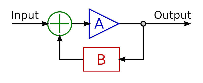
In the above diagram, Input (green) is the musical signal, which follows the arrows. A (blue) is the device. B (red) is a simple circuit that attenuates and inverts the output before feeding it back to the device input. The input to device (A) is the combination of the musical signal superimposed with an inverted portion of its own output.
You have now created a circuit or system whose response (Output) is the cumulative effect of the input signal, the device, and how the device responds to the combination of signal and negative feedback. This circuit has a linear response, even though the non-linear response of the device in the circuit has not changed.
Definitions: open loop is the device’s native response; closed loop is the response of the negative feedback circuit containing the device.
Open Loop Gain Feedback
Most devices have an open loop response that has (approximately) constant gain * bandwidth. This means in its output, amplitude * frequency is a constant. If frequency increases by a ratio of R, then amplitude (or gain) decreases by a ratio of R. This forms a linear slope dropping 20 dB per frequency decade. That’s because -20 dB is a ratio of 1:10, and a frequency decade is a ratio of 10:1, thus their product is constant (more on dB here).
For example, here is the gain-bandwidth curve for the AD797 opamp. It also shows phase which we aren’t discussing here, so I circled in red the gain-bandwidth curve. Note that it uses log scales on both axes (dB for Y, Hertz for X).
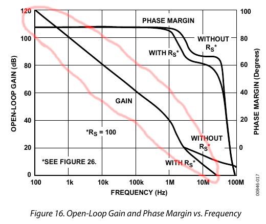
You can see that it drops almost exactly 20 dB per decade from 100 Hz to 1 MHz, then drops more steeply to 100 MHz. This is essentially the device’s native or “raw” frequency response.
This is a steep slope. If we take human hearing to be the range from 20 Hz to 20 kHz (not exact but a rough approximation), this is a ratio of 1000:1 which is 3 decades (10 * 10 * 10). Over this range, a device’s open loop response drops a whopping 60 dB! Intuitively, it amplifies low frequencies MUCH more than high frequencies. The AD797 is one of the cleanest best opamps for audio applications, yet clearly we must do something to correct its response before we can use it in an amplifier.
Non-Linearities
We said above that a device’s response is non-linear. A constant gain * bandwidth may be steeply sloped, but it is actually linear! So what part of the device is non-linear?
First, gain * bandwidth is not constant over the entire range of frequencies. Gain starts out flat, until reaching its first corner frequency where it begins to drop (below 100 Hz in the above graph, so not shown). This drop is not exactly linear, but only roughly so. Then it reaches its second corner frequency, where it drops faster (1 MHz in the above graph). Second, the device’s gain vs. amplitude is not linear either. That is, its gain ratio is not a constant – it responds differently to small versus large input signals. Both of these represent different kinds of distortion. Yet these examples are only 2 aspects of the more general concept of the device’s “transfer function“, which describes its output as a function of its input. The input to the transfer function is the musical signal. The output is the device’s response to that signal. The transfer function is not linear, not even close.
Finally, a device’s open loop gain is typically so large as to be unusable, like around 1 million to 1 (or 120 dB). For a usable amplifier, we need to reduce this gain down to roughly unity or 1:1. Sometimes less, sometimes more, but most audio applications are in the range of -30 to +30 dB. So we need something in the neighborhood of 100 dB of attenuation, or about 100,000:1.
This gives us 3 problems to solve before we can use a device as an audio amp:
- Flatten its steeply sloped frequency response.
- Reduce non-linearities in its transfer function (distortion).
- Reduce its unusably high gain ratio.
Negative feedback solves (or mitigates) all 3 of these problems. Essentially, it trades gain for linearity. In audio applications we have more open loop gain than we can use, which makes this an easy win-win trade.
Let’s take #3 first. Feeding the inverse of the device’s output back to its input obviously reduces gain. Indeed, the net effect would be zero, which is why we attenuate the negative feedback; we feed only a fraction of the output back to the input. It also makes the gain more stable. For example, suppose the device’s open loop gain changes with temperature. Negative feedback reflects any gain changes back to the input, offsetting them. If the device gain increased with temperature, the negative feedback gets more negative which shrinks the input accordingly, and vice versa). Closed loop gain no longer changes with temperature. Thus negative feedback reduces the device’s open loop gain (say, 1 million to 1) to whatever level you need (say, 1:1) and also makes it more stable.
Now consider #1: frequency response. If the device’s open loop gain-bandwidth curve looks like an inverted hockey stick, then its inverse looks like a right-side-up hockey stick. Feed this to the device input and the two curves cancel each other: you get a flat line. That is, constant gain versus frequency – otherwise called flat frequency response. This is true no matter what the shape of the device’s open loop gain-bandwidth curve – it doesn’t have to be linear.
Bandwidth is defined as the lowest frequency that sees a 3 dB drop in gain. If you have, say, 6 dB of negative feedback (half the output signal inverted and fed back to the input), the effect is like drawing a horizontal line across the device’s open loop gain-bandwidth chart, 6 dB below the top. Response is now flat from 0 moving to the right until it intersects the original gain-bandwidth curve.
For example, here (below, red line) is what the above device (AD797) frequency response would look like with 60 dB of negative feedback:
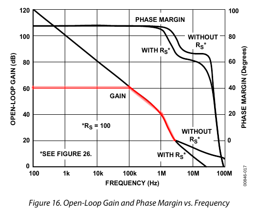
The circuit now has 60 dB of gain, instead of 120 dB, with flat frequency response to 100 kHz. We’ve traded 60 dB of gain for flatter frequency response (wider bandwidth), plus other benefits described below. And that’s still more gain than we need in most audio applications.
More negative feedback means a horizontal line further down on the chart, which is flat to a higher frequency before it intersects the open loop gain-bandwidth curve and starts to drop. Knowing that the open loop gain-bandwidth curve drops 20 dB per frequency decade, we can quantify this effect. Every 20 dB of negative feedback gives you about 10x more bandwidth. This is just a rough rule of thumb because it depends on the shape of the device’s gain-bandwidth curve, which as mentioned above is not perfectly linear.
This effect of applying complementary frequency response curves is similar to the RIAA EQ curve for vinyl LPs. Before cutting the record, they apply an EQ so that 20 Hz is 40 dB quieter than 20 kHz (roughly linear across the spectrum). On playback, they apply the reverse EQ boosting 20 Hz 40 dB more than 20 kHz. The 2 curves cancel each other, giving flat response.
Step 1 complete: negative feedback flattens the frequency response and determines the bandwidth.
As you go further down the chart, you get more bandwidth and less gain. At some point you’ll stop. This point is determined by:
- How much bandwidth you need
- How much gain you need
- How much gain & bandwidth you had to begin with (the device’s open loop gain-bandwidth curve)
Finally, consider step 2: distortion. This is merely a generalization of step 1. Negative feedback applies to the device’s transfer function; frequency response is only 1 aspect of that. By offsetting the transfer function, negative feedback corrects, reduces or squashes all non-linearities, for example distortion like harmonic and intermodulation.
In summary, we have explained how negative feedback achieves 3 goals:
- Flatten frequency response, widen bandwidth
- Reduce distortion
- Stabilize gain at a desired level
Timing & Phase
If negative feedback is delayed, then the negative waveform fed back to the input won’t line up with the device’s output. Thus, it can fail to offset the device’s transfer function, and may in some cases exaggerate it, turning into positive feedback. This is not normally a problem for audio, since audio frequencies are so low and slow compared to the device’s open loop bandwidth. However, if the gain-feedback loop has devices that alter the phase or have different impedance at different frequencies (capacitors or inductors), this could cause the same problem. Normally, the gain-feedback loop consists only of resistors to attenuate the signal to the desired level. In audio applications, metal film resistors are used due to their ideal noise profile.
In short, as long as the gain-feedback loop consists only of metal film or similar resistors, negative feedback should not introduce timing or phase issues in audio applications.
These Aren’t the Frequencies You’re Looking For
If you look at distortion specifications for amplifiers, you might notice that distortion usually rises with frequency. One reason for this is the shape of the device’s open loop gain-bandwidth curve. Its steep slope of -20 dB per decade means the device’s native output, and hence the negative feedback signal, consists mostly of low frequencies. This means low frequencies get more correction than high frequencies, which means lower distortion. Conversely, high frequencies have less feedback and consequently have higher distortion. Frequencies at the upper end of the bandwidth have almost no correction – they are so small in the device output, and thus also in the negative feedback.
This is the opposite of what we want because our hearing is much more sensitive to distortion in the middle to upper frequencies.
For example, highlighted in green in the diagram below, 60 dB of negative feedback as shown above gives us 60 dB of correction at 100 Hz, but only 15 dB of correction at 20 kHz. At 100 kHz where the red curve meets the black curve, the level of correction shrinks to zero.
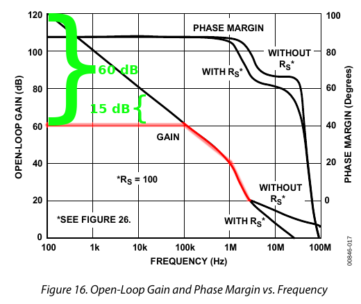
Here we’re talking about audio frequencies — kilohertz, not megahertz. Most devices have bandwidth into the megahertz range. A common solution is to use more negative feedback than you “need”, to make the bandwidth wider than the audio spectrum. This puts the highest audio frequencies in the middle of the bandwidth so they have enough feedback to reduce distortion. Of course, relatively speaking, they still have less feedback than the bass frequencies.