Category Archives: Audio

Analog vs. Digital

From Merriam Webster:

Analog

  1. of, relating to, or being a mechanism or device in which information is represented by continuously variable physical quantities
  2. something that is similar or comparable to something else either in general or in some specific detail : something that is analogous to something else

Digital

  1. composed of data in the form of especially binary digits
  2. of, relating to, or using calculation by numerical methods or by discrete units

In terms of storing, transmitting and playing audio, each term is ambiguous, yet their different meanings are similar, which leads to confusion.

Analog

The key phrase with meaning 1 is “continuously variable”. A turntable needle tracking a record groove, a tape deck head responding to fluctuating magnetic fields on tape, are both continuously variable. Reflective and non-reflective spots on a CD are not continuously variable – it either reflects a laser beamed at it, or it doesn’t. A square wave transmitted along a wire is not continuously variable – it is either at its max voltage, or its min voltage, nothing in between.

However, if we look more closely at the last two examples, we realize that they really are continuous. A reflective spot on a CD doesn’t reflect back 100% of the light; it’s not perfectly smooth, some of the light is scattered and lost. Conversely, a non-reflective spot does reflect back some tiny amount of the light, even though it absorbs or scatters most of it. And while all the spots of the same type (reflective or not) are similar, they are not exactly the same; each is unique. A square wave does not switch from high to low, or low to high, instantaneously. That would require infinite rise time, which is impossible. And as it approaches the new voltage, it will overshoot or undershoot just a bit before it stabilizes. So the voltage actually does vary continuously from the high to low value, even if it spends 99.99% of its time at a high or low value. In this sense neither of these are as discrete as they first seem; they are almost but not quite discrete, but actually continuous.

In fact, the universe at the super/macro scale at which we perceive and manipulate it, is continuous. It only becomes discrete at the micro/subatomic/quantum level.

The other sense of “analog” is that it is an “analog” of, or actually resembles the thing it represents (closely related to the word “analogy”). A magnetic tape that encodes music, has a strong field where the music is loud and a weaker field where it is quiet. A turntable needle tracking a record groove physically moves over a bigger amplitude when the music is loud, smaller when it is quiet. The shape of the groove itself resembles the waveform of the music being played.

Music as we experience it, and as it passes through air as vibrations and pressure changes, is continuously varying. Analog storage of music fulfills both definitions of the term: it is continuously varying, and it physically resembles the music (in some way, directly or indirectly).

Digital

The first definition refers to binary digits. However, this does not fully capture the sense of what it really means. The rational numbers are continuously varying, in the sense that they are infinitely dense: between any two of them, no matter how close they are, lie infinitely many more. Mathematically, the rational numbers are not a true “continuum”, as they have holes – by holes I mean numbers that we know must exist since they are the solution to simple algebra problems, yet are not rational. For example, the square root of 2.

Yet pragmatically speaking, this is a distinction without a difference. It is impossible to detect the difference between rational and real numbers through observation or measurement of the physical world. For every irrational number R, for any small value ε, we can pick a rational number Q so that | R – Q | < ε. We can pick ε smaller than any means of physical observation or measurement. Indeed, ε can be smaller than relativistic uncertainty principles permit. So even in theory, not just in practice, it is impossible to discern the difference in the physical universe. The difference between rational and real numbers does exist, but it is a mathematical distinction, not a physical one.

So for purposes of analog vs. digital, the notion of “infinitely dense” is a sufficient interpretation of what “continuous” means. Numbers can be continuous. Of course, numbers can also be non-continuous or discrete: like the counting numbers.

Even binary digits can be continuous. Every rational number can be expressed in binary digits, though some of them require infinitely many binary digits. For example, 1/7 in binary is 0.001001001… but that is still a well defined and valid number. When people use the term “binary digit” they often mean stored in a computer. But binary is simply a numbering system. It can be, but doesn’t have to be, stored in a computer.

However, in a computer the manifestation (storage, transmission, computation) of numbers is necessarily finite. Thus these numbers cannot be “infinitely dense”, which means they cannot be continuous. They are discrete numbers – even floating points, because they have finite resolution.

Because numbers can be either continuous or discrete, they are a poor concept on which to base the definition of “digital”. So much for Webster’s definition 1; that colloquial usage leads to confusion.

A better concept is definition 2: that of being “discrete units”. Storing or encoding data as a set of discrete states. We often use computers and binary, but the number of states is immaterial: it can be 2 (binary), 3 (trinary) or whatever.

In short, a big part of the confusion around the term “digital” is this: Just because it uses numbers, doesn’t mean it must be discrete. And just because it’s discrete, doesn’t mean it must use numbers.

Digital audio is discrete, and it uses numbers. The first is essential, the second is an incidental convenience.

Once again: truly discrete phenomena do not exist in our universe at the super-macro atomic scale. Discrete means a set of states with nothing in between the states. This is easy to understand from an abstract logical perspective. But shifting between physical states cannot be instantaneous, because that would require an infinite rate of change, which requires infinite energy/power.

Manifestation vs Meaning

Put differently: what it is vs what it means

Put differently: the signal, versus the information

A signal is a phenomena in the physical universe that encodes information. The signal can be a radio wave, a telephone transmission, handwriting on paper, scratches on a clay tablet, etc. Signals contain or encode information. The sender translates or encodes the information into the signal. The receiver decodes the information from the signal.

All signals are continuous, by the simple fact that they exist in our universe which does not have discrete phenomena at the macro/super scale. But this does not imply that all signals are “analogues” of the information they encode. Some are, some are not. That depends on the encoding.

The same signal could have different meaning, depending on the encoding. If the sender and receiver do not agree on the encoding, they may believe the message has been successfully transmitted, when it has not. The receiver might decode the signal in a different way than the sender encoded, and thus receive a different message.

This illustrates the fact that the signal, and the message or information it contains, are two different things. One is physical, the other logical. Signals cannot be discrete, but messages/information can be either discrete or continuous.

We can encode discrete messages into continuous signals. For example: consider the discrete binary message 11111100110 (which happens to be 2022, the current year). We can encode this into a series of voltage pulses each of fixed duration, encoding each 1 as 1.0 V and each 0 as -1.0 V. The receiver can easily extract the 1s and 0s from the signal.

However, somebody who doesn’t know the encoding scheme may receive this signal and not even know whether it contains a message, let alone what that message is.

Advantage: Digital

So what is the big deal behind digital audio? Why back in the 1980s was it called “perfect sound forever”? It’s neither perfect nor forever, so where did that phrase come from?

When encoding information into a signal, and decoding it from a signal, discrete states have certain advantages over continuous varying. Consider the above example of positive and negative voltage pulses. The receiver doesn’t care exactly what the voltage is. He can interpret any positive voltage as a 1, and any negative voltage as a 0. If the signal gets distorted, like a bunch of ripple added to it, or the peaks vary between 0.7 and 1.3 instead of exactly 1.0, it won’t change the message. The receiver will still receive it perfectly intact. Of course, under extreme conditions the signal could be so distorted that the message is lost, but that takes a lot of distortion. Encoding information as discrete states is robust, and in most normal cases delivers perfectly error-free messages.

Now consider an analog encoding of information, like a turntable needle tracking a record groove or a tape deck head detecting the magnetic field on tape passing by. Here, the encoding is continuously variable. Every tiniest wiggle or variation has meaning, it is part of the message. Indeed, high quality audiophile equipment is designed to respond to even those smallest subtle signal changes. If the signal gets distorted, even slightly, the distortion becomes part of the message. This encoding is not robust; it’s much more difficult to tell the difference between the encoded message, and any distortion that signal may have suffered.

Summary

For precision, let’s use “discrete” instead of “digital” and “continuous” instead of “analog”.

Digital audio is information. The original music is a continuous phenomena, and is encoded into information as discrete states. Those discrete states are encoded into continuous form for physical storage and transmission, and can be decoded back into discrete states. We use this discrete encoding because it is more robust, relatively immune from imperfections and distortions in transmission and storage, which makes possible perfect transmission that is not possible with information encoded in continuous forms.

In short, digital audio is “digital”, but the means by which we store and transmit it is “analog”. We encode the digital audio information into analog form or signals, and decode or extract the digital information from the analog signals.

The theory and physics of discrete vs. continuous information and signals has been known since Claude Shannon and others developed information theory back in the early 20th century. The Shannon-Whittaker interpolation formula which is the basis for analog to digital to analog conversion, was known at least since the 1930s. So why didn’t digital audio exist until the 1980s? The reason is computing power – or lack thereof. The range and resolution of human hearing is high enough that it requires a lot of digital data to attain sonic transparency. We knew how to do it, but it took decades for computing technology to get fast enough to process the volume of digital data required.
Negative Feedback

Introduction

I’m not talking about people complaining about stuff.  This is about feedback in amplifiers. I first heard about this back in the 1980s when I got into this hobby, but I never understood it as well as I wanted to. I think this is true of many other audiophiles. Most of the textbooks and other literature discussing negative feedback is either so technical it’s hard for people without EE degrees to understand (I took some EE classes but my degree is in Math), or it’s so high level it amounts to hand-waving. Over time I’ve studied it more closely and gradually understood it better. I thought this intuitive description may give the fundamental understanding needed to then go off and read the more technical stuff.

Opamps and transistors (henceforth, “devices”) are used to amplify signals – in our case as audiophiles, music. But they do not have linear outputs, not even close. This applies to their output in both frequency and amplitude domains. Non-linearities are distortion, in one form or another.

Negative Feedback: Definition

Negative feedback is a method to make these devices more linear.

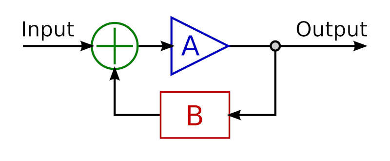
The concept is simple: feed the device output back to its input, inverted. Some portion or % of the device output is inverted and fed back to the input. Hence the name: Negative means it is inverted, Feedback means it’s fed back to its input. Here’s a simple negative feedback circuit:
In the above diagram, Input (green) is the musical signal, which follows the arrows. A (blue) is the device. B (red) is a simple circuit that attenuates and inverts the output before feeding it back to the device input. The input to device (A) is the combination of the musical signal superimposed with an inverted portion of its own output.

You have now created a circuit or system whose response (Output) is the cumulative effect of the input signal, the device, and how the device responds to the combination of signal and negative feedback. This circuit as a whole has closer to linear response, even though the non-linear response of the device in the circuit has not changed.
Definitions: open loop is the device’s native response without negative feedback; closed loop is the response of the negative feedback circuit containing the device.
Open Loop Gain Feedback

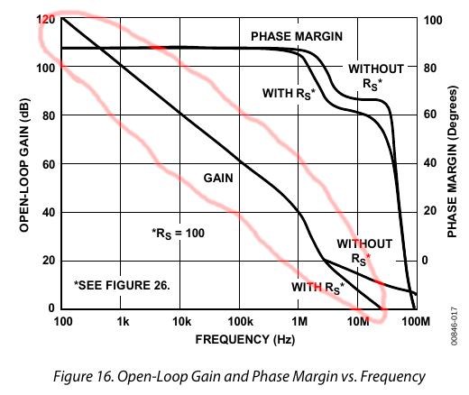
Most devices have an open loop response that has (approximately) constant gain * bandwidth. This means in its output, amplitude * frequency is a constant. If frequency increases by a ratio of R, then amplitude (or gain) decreases by a ratio of R. This forms a linear slope dropping 20 dB per frequency decade. That’s because -20 dB is a ratio of 1:10, and a frequency decade is a ratio of 10:1, thus their product is constant (more on dB here).

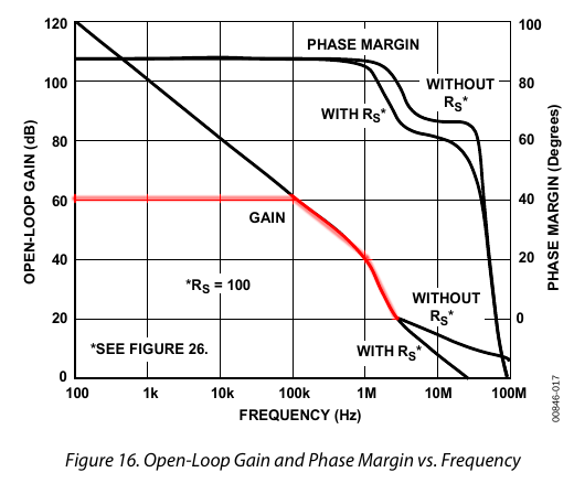
For example, here is the gain-bandwidth curve for the AD797 opamp. It also shows phase which we aren’t discussing here, so I circled in red the gain-bandwidth curve. Note that it uses log scales on both axes (dB for Y, Hertz for X).

You can see that it drops almost exactly 20 dB per decade from 100 Hz to 1 MHz, then drops more steeply to 100 MHz. This is essentially the device’s native or “raw” frequency response.

This is a steep slope. If we take human hearing to be the range from 20 Hz to 20 kHz (not exact but a rough approximation), this is a ratio of 1000:1 which is 3 decades (10 * 10 * 10). Over this range, a device’s open loop response drops a whopping 60 dB! Intuitively, it amplifies low frequencies MUCH more than high frequencies. The AD797 is one of the cleanest best opamps for audio applications, yet clearly we must do something to correct its response before we can use it in an amplifier.

Non-Linearities

We said above that a device’s response is non-linear. A constant gain * bandwidth may be steeply sloped, but it is actually linear! So what part of the device is non-linear?

First, gain * bandwidth is not constant over the entire range of frequencies. It is approximately linear in the middle of its range, but non-linear at low and high frequencies. Second, the device’s gain vs. amplitude is not linear either. That is, its gain ratio is not a constant – it responds differently to small versus large input signals. Both of these represent different kinds of distortion. Yet these examples are only 2 aspects of the more general concept of the device’s “transfer function“, which describes its output as a function of its input. The input to the transfer function is the musical signal. The output is the device’s response to that signal. The open loop transfer function is not linear, not even close.

Finally, a device’s open loop gain is typically so large as to be unusable, like around 1 million to 1 (or 120 dB). For a usable amplifier, we need to reduce this gain down to roughly unity or 1:1. Sometimes less, sometimes more, but most audio applications are in the range of -30 to +30 dB. So we need something in the neighborhood of 100 dB of attenuation, or about 100,000:1.

This gives us 3 problems to solve before we can use a device as an audio amp:

  1. Flatten its steeply sloped frequency response.
  2. Reduce non-linearities in its transfer function (distortion).
  3. Reduce its unusably high gain ratio.

Negative feedback solves (or mitigates) all 3 of these problems. Essentially, it trades gain for linearity. In audio applications we have more open loop gain than we can use, which makes this an easy win-win trade.

Let’s take #3 first. Feeding the inverse of the device’s output back to its input obviously reduces gain. Indeed, the net effect would be zero, which is why we attenuate the negative feedback; we feed only a fraction of the output back to the input. It also makes the gain more stable. For example, suppose the device’s open loop gain changes with temperature. Negative feedback reflects any gain changes back to the input, offsetting them. If the device gain increased with temperature, the negative feedback gets more negative which shrinks the input accordingly, and vice versa). Closed loop gain no longer changes with temperature. Thus negative feedback reduces the device’s open loop gain (say, 1 million to 1) to whatever level you need (say, 1:1) and also makes it more stable.

Now consider #1: frequency response. If the device’s open loop gain-bandwidth curve looks like an inverted hockey stick, then its inverse looks like a right-side-up hockey stick. Put differently: the biggest frequencies in the output, when inverted, will have the biggest attenuation. Feed this to the device input and the two cancel each other: you get a flat line. That is, constant gain versus frequency – otherwise called flat frequency response. This is true no matter what the shape of the device’s open loop gain-bandwidth curve – it doesn’t have to be linear.

Bandwidth is defined as the lowest frequency that sees a 3 dB drop in gain. If you have, say, 6 dB of negative feedback (half the output signal inverted and fed back to the input), the effect is like drawing a horizontal line across the device’s open loop gain-bandwidth chart, 6 dB  below the top. Response is now flat from 0 moving to the right until it intersects the original gain-bandwidth curve.

For example, here (below, red line) is what the above device (AD797) frequency response would look like with 60 dB of negative feedback:

The circuit now has 60 dB of gain, instead of 120 dB, with flat frequency response to 100 kHz. We’ve traded 60 dB of gain for flatter frequency response (wider bandwidth), plus other benefits described below. And that’s still more gain than we need in most audio applications.

More negative feedback means a horizontal line further down on the chart, which is flat to a higher frequency before it intersects the open loop gain-bandwidth curve and starts to drop. Knowing that the open loop gain-bandwidth curve drops 20 dB per frequency decade, we can quantify this effect. Every 20 dB of negative feedback gives you about 10x more bandwidth. This is just a rough rule of thumb because it depends on the shape of the device’s gain-bandwidth curve, which as mentioned above is not perfectly linear.

This effect of applying complementary frequency response curves is similar to the RIAA EQ curve for vinyl LPs. Before cutting the record, they apply an EQ so that 20 Hz is 40 dB quieter than 20 kHz (roughly linear across the spectrum). On playback, they apply the reverse EQ boosting 20 Hz 40 dB more than 20 kHz. The 2 curves cancel each other, giving flat response.

Step 1 complete: negative feedback flattens the frequency response and determines the bandwidth.

As you go further down the chart, you get more bandwidth and less gain. At some point you’ll stop. This point is determined by:

  • How much bandwidth you need
  • How much gain you need
  • How much gain & bandwidth you had to begin with (the device’s open loop gain-bandwidth curve)

Finally, consider step 2: distortion. This is merely a generalization of step 1. Negative feedback applies to the device’s transfer function; frequency response is only one aspect of that. By offsetting the transfer function, negative feedback corrects, reduces or squashes all non-linearities, for example distortion like harmonic and intermodulation.

In summary, we have explained how negative feedback achieves 3 goals:

  1. Flatten frequency response, widen bandwidth
  2. Reduce distortion
  3. Stabilize gain at a desired level

Timing & Phase

If negative feedback is delayed and the input signal is changing (like music), then the negative waveform fed back to the input won’t line up with the device’s output. Thus, it can fail to offset the device’s transfer function, and may in some cases exaggerate it, turning into positive feedback. This is not normally a problem for audio, since audio frequencies are so low and slow compared to the device’s open loop bandwidth. However, if the gain-feedback loop has devices that alter the phase or have different impedance at different frequencies (capacitors or inductors), this could cause the same problem. Normally, the gain-feedback loop consists only of resistors to attenuate the signal to the desired level. In audio applications, metal film resistors are often used due to their ideal noise profile and resistance characteristics (low inductance & capacitance).

In short, as long as the gain-feedback loop consists only of clean resistors, negative feedback should not introduce timing or phase issues in audio applications.

These Aren’t the Frequencies You’re Looking For

If you look at distortion specifications for amplifiers, you might notice that distortion usually rises with frequency. One reason for this is the shape of the device’s open loop gain-bandwidth curve. Its steep slope of -20 dB per decade means the device’s native output, and hence the negative feedback signal, consists mostly of low frequencies. This means low frequencies get more correction than high frequencies, which means lower distortion. Conversely, high frequencies have less feedback and consequently have higher distortion. Frequencies at the upper end of the bandwidth have almost no correction – they are so small in the device output, and thus also in the negative feedback.

This is the opposite of what we want because our hearing is much more sensitive to distortion in the middle to upper frequencies.

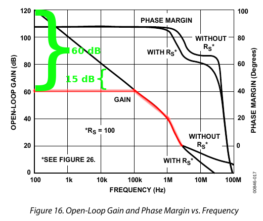
For example, highlighted in green in the diagram below, 60 dB of negative feedback as shown above gives us 60 dB of correction at 100 Hz, but only 15 dB of correction at 20 kHz. At 100 kHz where the red curve meets the black curve, the level of correction shrinks to zero.

Here we’re talking about audio frequencies — kilohertz, not megahertz. Most devices have bandwidth into the megahertz range. A common solution is to use more negative feedback than you “need”, to make the bandwidth wider than the audio spectrum. This puts the highest audio frequencies in the middle of the bandwidth so they have enough feedback to reduce distortion. Of course, relatively speaking, they still have less feedback than the bass frequencies.

SMSL SU-6 Review: DAC + Preamp

Introduction

I’ve said this before but it’s worth repeating: when it comes to audio, we are spoiled with an abundance of riches. DACs, amps, headphones have gotten so much better over the past 15 years, it’s hard to imagine that this was sometimes considered a “solved problem”. At the same time, prices have gone down, not up.

A few weeks ago I got a Topping EX5. It was a great little device but it had buggy software and Topping could not fix it. So I got an SMSL SU-6 to see if would be any better. Amir reviewed the SMSL SU-6 favorably at ASR. Refer there for detailed measurements.

Here I’ll fill in some of the details that Amir doesn’t cover: whether the SU-6 has the same software bugs as the EX5 (or others), and details on its digital filters.

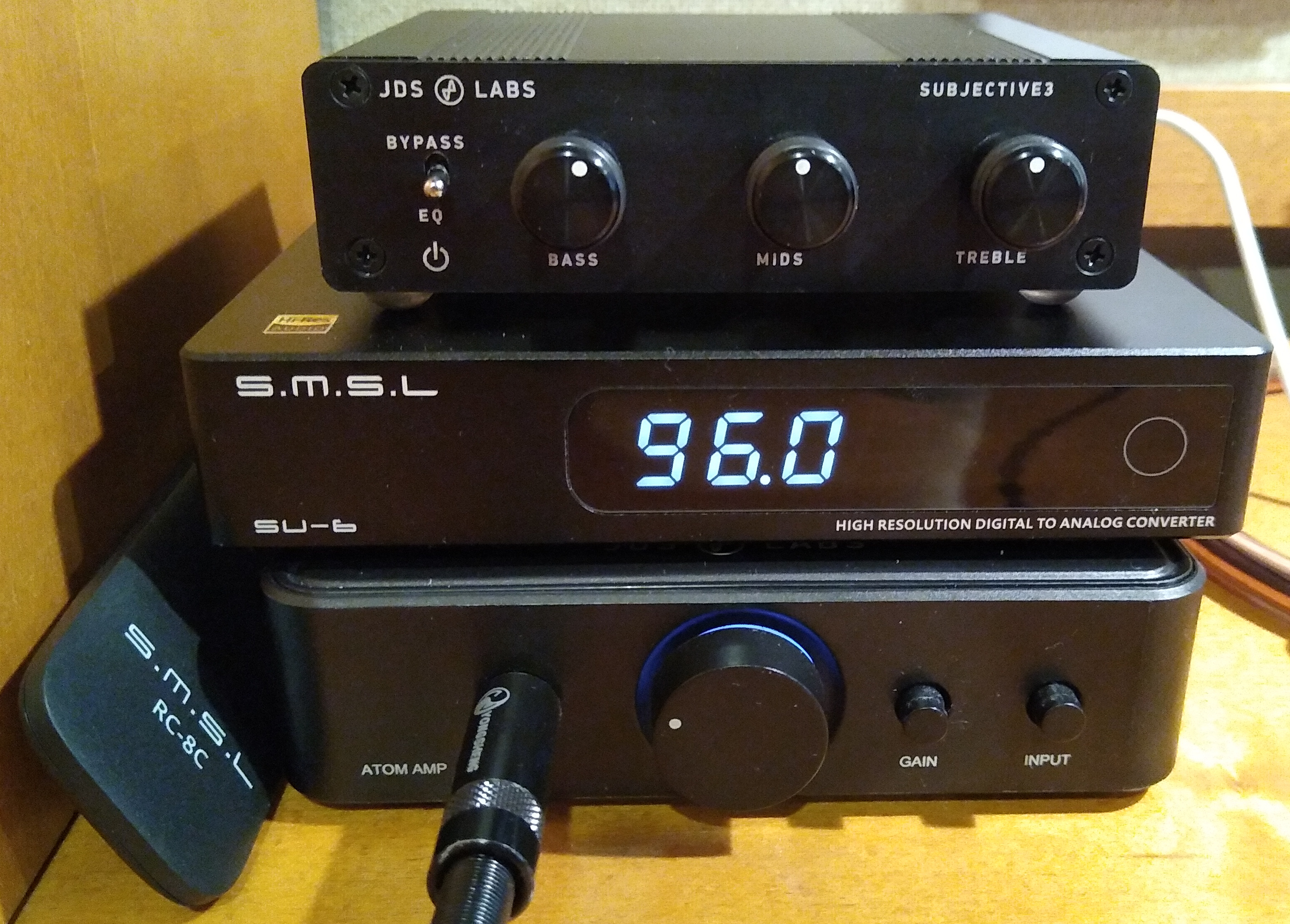
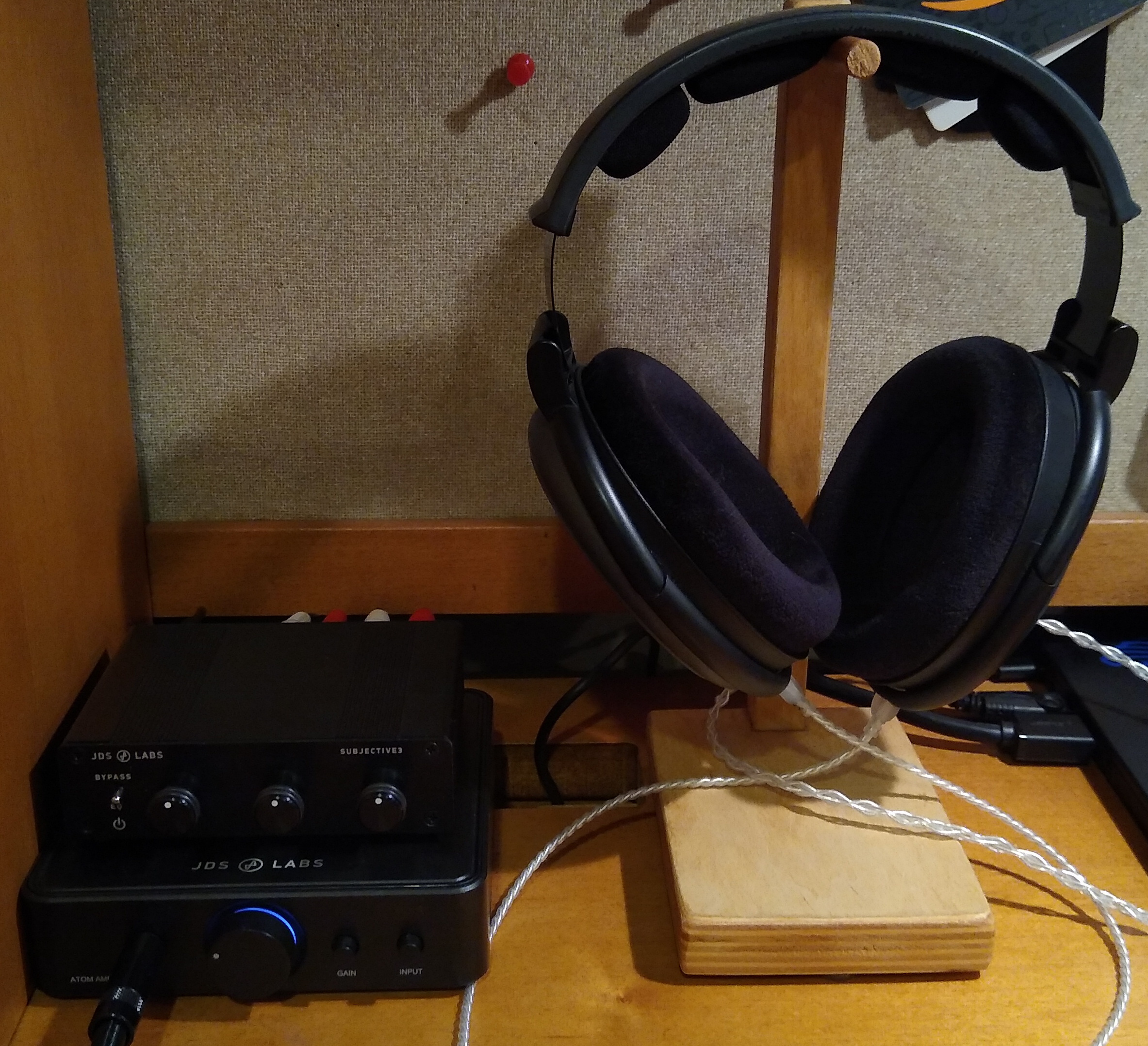
Here’s what the SU-6 looks like in service – my computer desktop audio stack: the SMSL SU-6, the JDS Subjective 3 EQ, and the JDS Atom headphone amp. The slight bass boost compensates for the Sennheiser HD-580 bass rolloff.

Summary

TLDR: The SMSL SU-6 is simpler than the EX5. It is a single-ended, line-level DAC, only that and nothing more. No headphone amp, no balanced outputs. It does have a volume control. I bought it for $170 on Amazon. This is my second piece of “Chi-Fi” (Chinese Hi-Fi) equipment, the EX5 being the first.

Compared with other well engineered DACs having excellent measured performance, what distinguishes the SU-6?

  • Display properly shows current sample rate
  • Volume control, useful to turn it down a few dB to avoid clipping hot sources
  • Several digital filters from which to pick
  • Adjustable phase lock to minimize jitter and prevent audio glitches
  • Internal power supply – no wall wart

Update: Feb 2023

My SU-6 which has been reliable for just over a year, just developed a problem. I was listening yesterday and it didn’t sound quite right. Too subtle to pin down, so I measured it. It has developed THD at -55 to -60 dB, all 2nd harmonic. It used to measure clean (THD below 90 dB which is what my sound card measures in loopback mode). I got in touch with SMSL support via email and the outcome is pending. As I check reviews on Amazon, it seems the SU-6 has more than its fair share of failures and support can be difficult.

Resolution

Support was difficult to contact and led to a frustratingly slow drawn out email chain with people having limited English language skills. Finally they agreed I could send it back for repair, but I chose not to:

  • I have to pay to ship it to them for repair.
  • Mailing packages to China is prohibitively expensive.
  • There’s no guarantee it will arrive, could get held up or lost in customs.
  • If it does arrive, there’s no guarantee the company will actually fix it. The unit was 100% functional but had slightly distorted analog output. They might do a simple function check and return it as “nothing to fix”.
  • If they do actually fix or replace it, there’s no guarantee it will arrive back home. It could get held up or lost in customs.

For these reasons, I considered it a $190 lesson and opted not to take risk of throwing good money after bad. This means I needed (haha, I use that word loosely) a new DAC. And after my bad experiences with Topping and SMSL, no more Chi-Fi for me. It’s not worth the risk and hassles. I’ll buy gear from the USA, Japan or Germany for the quality and support.

Back to the Review

Good Stuff

  • Excellent measured performance
  • Great subjective sound quality: clean, detailed, neutral
  • Seamless operation – no software bugs encountered
  • Functionally complete: several digital inputs, useful firmware settings
  • Simple: no controls,  switches or moving parts that can eventually fail
  • Internal power supply – no wall wart
  • Solid build quality
  • Low price

Bad Stuff

  • Single-ended only (no balanced outputs)
  • Line-level only (no headphone amp)
  • Questionable reliability / longevity
  • Poor warranty & support

Overview

First, check out Amir’s detailed measurements on ASR. The SU-6 is a well engineered device and one of the best measuring DACs.

What is the SU-6?

  • DAC supporting PCM and DSD formats
  • Select between 4 inputs
  • Volume control
  • Preamp (line-level single-ended output with volume control)

The SU-6 has 4 inputs, all digital:

  • USB (async/pull)
  • SPDIF (coax and toslink)
  • Bluetooth

Key SU-6 Features

  • Reference quality audio: digital & analog
  • Internal power supply: no wall-wart
  • Digital volume control
    • Perfect channel balance at all levels
    • Preserves high SNR even at low volumes
  • Display shows current sample rate (useful for troubleshooting/confirming)
  • User-selectable digital filters: choose from 7!
    • linear vs. minimum phase
    • sharp vs. slow attenuation
  • User-selectable sample rate sync timing

Case, Knobs & Quality

Overall the SU-6 is a cute little plastic and metal box. And it is little: 5 1/2″ wide, 4″ deep, 1″ high. The connectors feel solid, the display has 5 brightness levels and is evenly lit. Volume is controlled only by remote; there is no knob. To me, this is not a deficiency but a feature since knobs eventually fail, and I wouldn’t use it anyway, as I leave the SU-6 volume set to -12 (-6 dB, to avoid clipping loud content having intersample overs) and control volume with my headphone amp.

In use, the SU-6 doesn’t get warm, but only slightly above room temperature. It has a single capacitive touch button that selects the input. All other functions are controlled by the remote. The SU-6’s only moving part is the power switch in the back.

Volume Control

The SU-6 has a volume control with 100 steps. To assess how the steps interact with volume level, I measured the output level using white noise. The top 70 steps drop by 1/2 dB each (volume setting -70 is -35 dB) and the rest of the steps get progressively bigger until the penultimate step (-98) which is  -71 dB, and the lowest step (-99) mutes entirely.

Settings

Besides volume, the SU-6 has 3 settings controllable from the remote:

  • Digital filters: 1 through 7
  • Sample rate phase lock: 1 through 9
  • Screen brightness: 1 through 5
Digital Filters

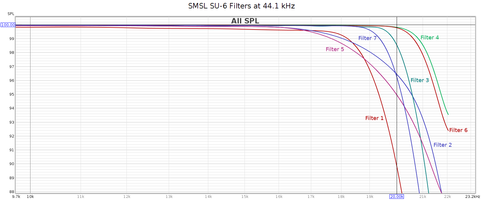
The SU-6 has 7 digital filters. TLDR; filter #3 and #6 are the best (flattest frequency & phase response), and filter #4 is the best minimum phase / causal / asymmetric. The filter responses match the descriptions in the manual.

Here’s what I got when I measured them:

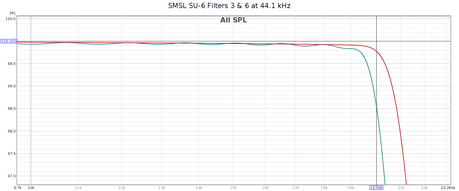
Here’s a close-up comparison of filters #3 and #6:

I recommend #6, but filter #3 is a good alternative. Filter 6 has the widest, flattest, smoothest passband response. Its only drawback is that it doesn’t fully attenuate by Nyquist (22,050 Hz). It reaches full attenuation by 24,100 Hz. This leaks HF noise, but it should be benign as all aliases must be > 20 kHz (inaudible). Filter 3 fully attenuates by Nyquist, but in order to do that, it has some passband attenuation (-1.5 dB @ 20 kHz) and ripple (0.1 dB). Both are quite small and inaudible to most people. Some people prefer minimum phase / causal / asymmetric impulse filters. The best such filter in the SU-65 is filter #4.

This goes to show that the CD redbook standard of 44.1-16 is not really sufficient for complete transparency. The sample rate is just a bit too low, making such a narrow transition band that even the best DAC chips (the SU-6 uses the ESS-9038) are not both correct and transparent. And while 16 bits / 93 dB of dynamic range is sufficient for most music, it falls short of the full dynamic range of our hearing. What we really need for complete transparency is at least 48 kHz / 24-bit. This is already a standard with DVD, why not make it the new standard for music too? This would actually simplify things as everything (both movies & music) would use the same format.

Sample Rate Phase Lock

SPDIF is a “push” protocol for digital audio. This means the source delivers audio data and the destination/receiver (the DAC) must synchronize with the source. The problem here is that the source (audio player) & receiver (DAC) each has its own independent clock, and no 2 clocks ever agree exactly. It is not enough for the receiver to buffer and re-clock the received data, because if the clocks don’t exactly match, the buffer will eventually under- or over- flow. So the receiver must compute the average rate at which data arrives, to detect the sample rate in terms of its own clock, use that sample rate even if it isn’t exactly what it’s supposed to be, and constantly re-compute and adjust as it runs.

For example, consider 44.1 kHz sampling. If the clocks are off by 1 part in 1 million, that’s 1 sample every 22.6 seconds. In this case, the DAC must detect this and adjust its clock rate to 44,099.999999 or 44,100.000001.

The SU-6 has a setting to adjust how it does this, a range from 1 to 9. The best sound quality (value 1) is the least permissive of clock differences. This has immeasurable jitter but it will glitch if the clocks don’t match nearly perfectly. Value 9 is the most permissive setting, so it can handle more clock rate variance without glitching. Yet it is more subject to jitter.

How to pick the best setting? Start with #1. If that works, you’re done. If it glitches, increase it step by step until it doesn’t glitch.

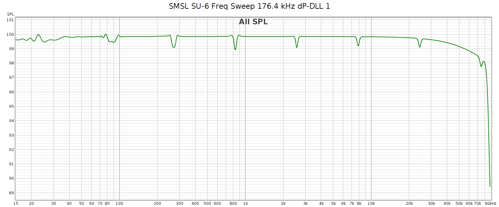
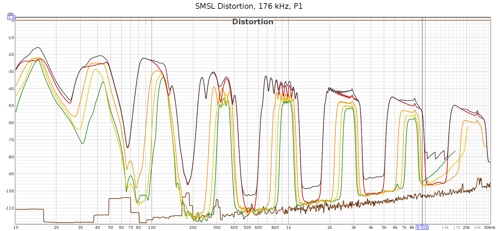
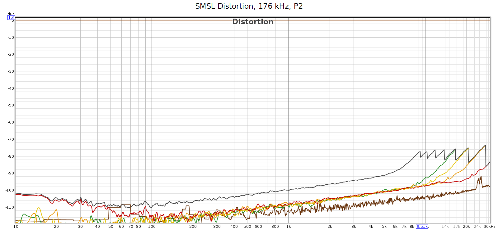
If all this sounds theoretical, for those who believe digital audio jitter is a non-issue, consider what I encountered when testing the SU-6. I played frequency sweeps at sample rates 44.1, 48, 88.2, 96, 176.4 and 192 kHz. All of them were smooth and clean except for 176.4, which had a few audible “tics” every time I played it. The sweep looked like this:Distortion measured like this:No question this is audible distortion.

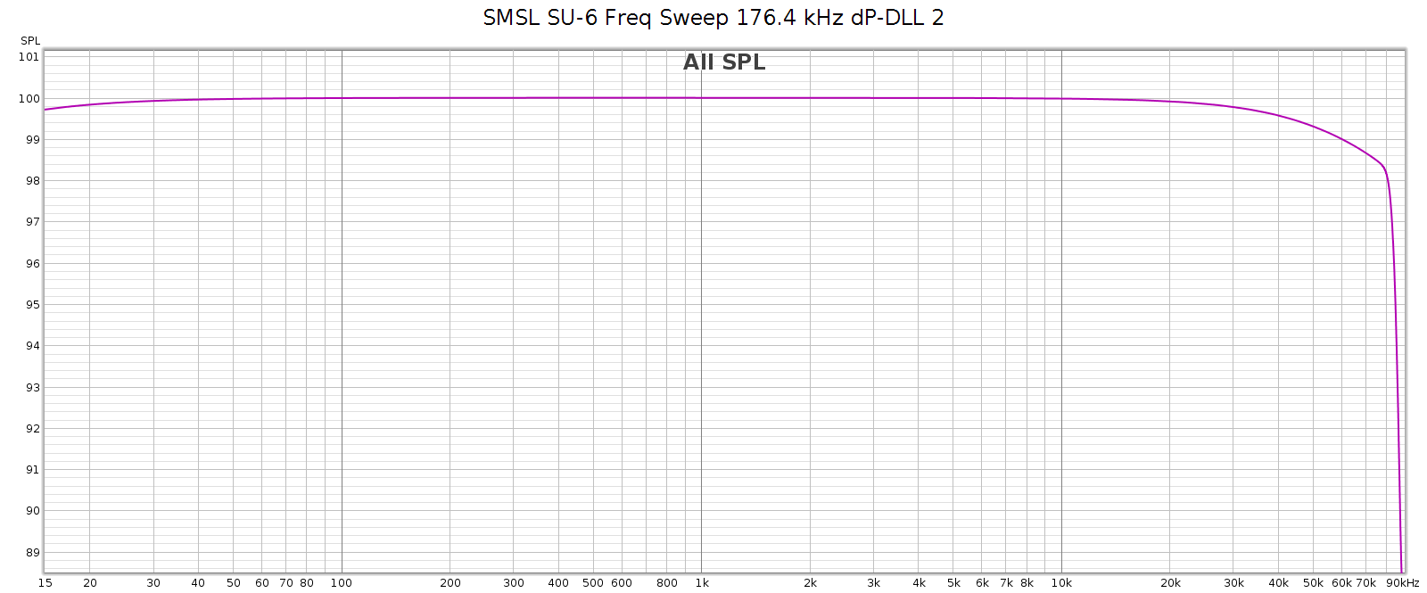
After re-testing and troubleshooting, I couldn’t figure out what the problem was. Then I RTFM and discovered the dP-DLL setting. I increased it from 1 to 2, re-tested and the “tics” were gone. It measured clean, like all the other sample rates:The distortion was gone too, now showing only the distortion from my sound card:

It was cool and satisfying to actually find a problem bench testing this device, then find a way to fix it. Yes, the dP-DLL setting actually does make a difference! And through bench testing I was able to confidently find the best digital filter.

Brahms Symphony 3: High Def Recording Analysis

Introduction

I was listening on Qobuz to this recording of Ivan Fischer conducting the Budapest Festival Orchestra playing Brahms Symphony 3. It happens to be a 192k – 24 bit recording. This recording sounded a bit “off” but I couldn’t place exactly why. So I captured the bitstream and here’s what I found.

The Capture

First: this capture consists of a single brief section of the recording purely for educational use and is not distributed. This places it under “fair use” for copyright.

I captured the opening of the 1st movement, which starts with about 1 second of room silence then the orchestra starts at medium volume. When I opened the audio file in Audacity, I noticed the wave didn’t show any obvious change in amplitude when the orchestra started. It looked like this:

Perceptually, it was quiet for the first second before the orchestra played. But this audio file shows the room silence at only 30 dB below peak levels, which is much too loud.

The Solution

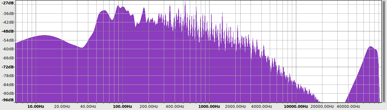
Aha! I thought, perhaps this is ultrasonic noise! A spectrum analysis showed this to be the case:

This is an obvious glaring flaw in this recording. We have supersonic noise peaking at 70-80 kHz, just below the 192 kHz Nyquist limit. It’s so loud, it’s at the same level as easily audible 4 kHz audio content!

I could easily fix this in 2 ways: apply a low pass filter or resample it at a lower rate. The first step of down-sampling would apply a low pass filter, and this recording didn’t need to be at 192 kHz anyway. So I resampled it to 96 kHz. The half-rate integer multiple keeps the resampling method computationally simpler and cleaner. I could have down-sampled 4:1 to 48 kHz, but 96 kHz would be sufficient, as most of the noise was above 48 kHz.

The Result

Here’s the resulting wave file:

The room silence opening is now at least 50 dB below peak, which is typical.

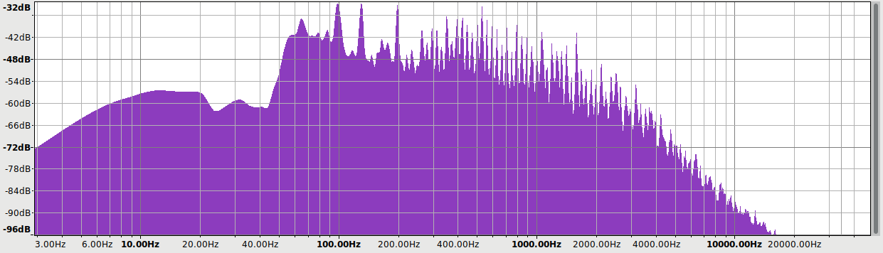
The spectrum analysis:

The supersonic noise has been eliminated.

It is a bit unnerving that a professional recording can get released with such a serious flaw. Yet I noticed that this recording on Presto Classical is available at most 96 kHz, not 192. Could it be this problem was introduced by Qobuz processing it for streaming? Probably not, as Qobuz says they stream whatever the studios give them, without changing it. Supersonic noise in that spectrum almost certainly didn’t come from the room or the mics. It was most likely introduced by an improper format conversion from the original DSD to 192 kHz PCM. I don’t know why it sounded “off” since the high frequency noise should have been inaudible. Perhaps it was interacting with passband frequencies, causing audible intermodulation distortion. Or perhaps it was the result of improper low pass filtering, which also caused aliasing in the passband. Whatever the root cause, it was fun and educational to explore, and shows that recording studios sometimes make mistakes.

Topping EX5 Review: DAC+ Preamp + Headphone Amp

Introduction

When it comes to audio, we are spoiled with an abundance of riches. DACs, amps, headphones have gotten so much better over the past 15 years, it’s hard to imagine that this was sometimes considered a “solved problem”. At the same time, prices have gotten incredibly low.

For example, 15 years ago if you wanted a DAC + headphone amp having studio reference quality, the Benchmark DAC or Grace M920 were two of your only options, both cost $1 – $2 kilobucks which would be about 50% more in today’s dollars. Back in ’99 I bought a Headroom Maxed out Home amplifier that cost $1000. It was the best headphone amp of its time, both in measurements and subjective listening. Today for $150 you can get amps having even cleaner measurements and more power. That’s only 1/10 of the inflation adjusted equivalent price.

Summary

TLDR: The Topping EX5 is functionally comparable to those Benchmark and Grace devices, and equal or superior in terms of measurements. It retails for $350, I bought it on sale for $300, which is about 1/10 of their equivalent price. This is my first piece of “Chi-Fi” (Chinese Hi-Fi) equipment. Here are my impressions having used it daily for a few weeks, including bench testing with Room EQ Wizard.

Good Stuff

  • Excellent measured performance
  • Great subjective sound quality: clean, detailed, neutral
  • Solid build quality
  • Low price

Bad Stuff

  • The manual has serious errors (mislabeled digital filters)
  • Factory support is poor to entirely lacking (no responses to support queries)
  • It has obvious software bugs (the display shows the wrong sampling rate)

Those last 2 are double-threat. I can live with software bugs if the company has great support, as they will fix the bugs. I can live with poor support if the device works seamlessly, as I won’t need support. But a buggy device combined with poor support is a “no-go” for me.

Overview

First, check out Amir’s detailed review & measurements on ASR. The EX5 is a well engineered device having excellent measured performance.

What is the EX5?

  • DAC supporting PCM and DSD formats
  • Select between 4 inputs
  • Volume control
  • Line-level preamp
  • Headphone amp

Inputs:

  • SPDIF Coax
  • SPDIF Toslink
  • USB
  • Bluetooth

Outputs:

  • Line: Balanced XLR and SE RCA
  • Headphone: Balanced 4-pin and SE 1/4″ plug

Key EX5 features

  • Compact all-in-one device: DAC, preamp, headphone amp
  • Reference quality audio: digital & analog
  • Internal power supply: no wall-wart
  • Digital volume control
    • Perfect channel balance at all levels
    • Preserves high SNR even at low volumes: 90 dB SNR @ 50 mV
  • User-selectable digital filters: choose from 7!
    • linear vs. minimum phase
    • sharp vs. slow attenuation


Case, Knobs & Quality

Overall the EX5 feels like a high quality piece of kit. The case is heavy & neat, the connectors feel solid, the display is evenly lit, the volume knob has a smooth clicky feel.

The volume knob is a rotary encoder that also serves as a push-button. I’ve seen rotary encoders start to fail in other equipment I own. After a few years their click action became glitchy, as you turn it up it sometimes turns down, etc. Cleaning the internal contacts with electrical spray helps but is temporary as the problem eventually recurs. I hope the EX5 rotary encoder does not suffer the same fate.

The display has 3 brightness levels and is always on. It has an auto-dim feature in which the display goes mostly dark after 30 seconds, showing only the selecting input. This is my preferred mode, as it hides the incorrect display of sample rate.

In use, the EX5 gets warm but not hot. Just a touch warmer than my JDS Atom amp. The EX5 case is solid metal with no vents on the bottom, sides or top. It feels like the solid metal case serves to dissipate its internal heat.

Volume Control

The EX5 has 2 gain modes: low (standard) and high, which is 10 dB louder. Its volume control has 100 steps. To assess how the steps interact with volume level, I measured the output level using white noise:

  • 100: max
  • 60: -20 dB
    • From 60 – 100, each step is 1/2 dB
  • 30: -50 dB
    • From 30 – 60, each step is 1 dB
  • 20: -68 dB

Low gain has plenty of volume for my HD-580 and LCD-2F headphones. I typically listen around setting 50-60 with high dynamic range music having low average levels. This is about 30 dB below max. So I’d be using lower levels for rock or modern music which is dynamically compressed having louder average levels.

Note: at low gain, 0 dB is 4.1 Vrms. Volume setting 50 is 30 dB quieter, which is 3.16% of that, or 130 mV. This drives the LCD-2F to 87.5 dB SPL for the loudest peaks of the music. But it’s really 6 dB quieter because my DSP for EQ drops the overall levels by 6 dB. So my typical listening puts the loudest musical peaks at around 82 dB SPL.

Wish List

The EX5 packs a lot of functionality in a compact box. Yet the challenge of single-box audio devices is they can work so well they leave me wanting just a bit more. Here’s what I wish the EX5 also did…

DSP

It would be great to have parametric EQ and crossfeed for headphones. Of course, it would take some creative thinking to do this with the EX5’s single knob/button. Without it, you must find a way to apply whatever DSP you want, upstream from the EX5.

Analog Input

The title speaks for itself. The EX5 has a great little built-in preamp / headphone amp and it would be really useful to have an analog input. Yet I understand why they didn’t do this. Since the EX5 has a digital volume control, they would have to significantly change the device in order to accept analog inputs.

Bugs / Problems

No device is perfect. Here are the issues I found with the EX5.

Sample Rate Display

The biggest problem I found with the EX5 is the display. When using SPDIF input over toslink or coax, the display always shows 44.1 (sometimes 48) regardless of the actual sample rate. Sometimes it shows the right sample rate, usually it does not and gets stuck at 44.1. For example, I measured the EX5 at 44.1, 48, 88.2, 96, 176.4 and 192. For the entire time the display showed 44.1 even when it was clearly operating at these other rates. As I type these words I’m listening to Sibelius Symphony #1 at 96 kHz yet the EX5 display is showing 44.1. One when I played 96k content the display showed 48.

This happens over digital coax or toslink from my Juli@ sound card, and over the toslink output of my Behringer DEQ2496. My other DACs (Oppo HA-1 and Corda Soul) show the proper sample rate from these devices.

I reported this to Topping on their support web site and got no reply. And tagged them on the ASR forum, no reply. There is essentially no factory support for this device.

I speculate that Topping designed this device to be plugged into Windows or Mac computers, and they rely on their custom device driver to set the displayed sample rate. In other words, the EX5 doesn’t show you the actual sample rate at which it is working, it shows you whatever rate the driver tells it to display, and defaults to 44.1 or 48.

Auto-Mute

The EX5 auto-mutes if the digital audio input has a quiet L channel. The delay depends on sample rate: about 5 secs at 192k, about 25 secs at 44.1k. This is not documented and could cause frustrating lost time chasing down ghosts if you don’t know about it.

Balanced – Not Really

The EX5 has balanced outputs, both line (XLR) and headphone (4-pin). The XLR line out has twice the voltage of the RCA (4.3 Vrms vs. 2.1), so it appears to be fully balanced (differentially signalled). But the headphone output has the same voltage output on either (5.9 Vpp with low gain, 18.3 Vpp on high), so it’s not fully balanced. The balanced headphone outputs probably use separate grounds for the L and R channels, as the balanced channel separation is higher (99 vs. 88 dB).

Note: the headphone output is given as Vpp, so multiply by 0.7 to get Vrms. Thus for low gain, 5.9 Vpp –> 4.1 Vrms and for high gain, 18.3 Vpp –> 12.6 Vrms.

Measurements

I measured the EX5 using Room EQ Wizard and my Juli@ PC sound card. This equipment is pretty basic so I can’t measure the full extent of the EX5 sound quality. But it does enable me to test some of the basics.

Here I will focus on frequency response and the digital filters. This is for 2 reasons:

  1. The EX5 manual is wrong
  2. This is easy to measure

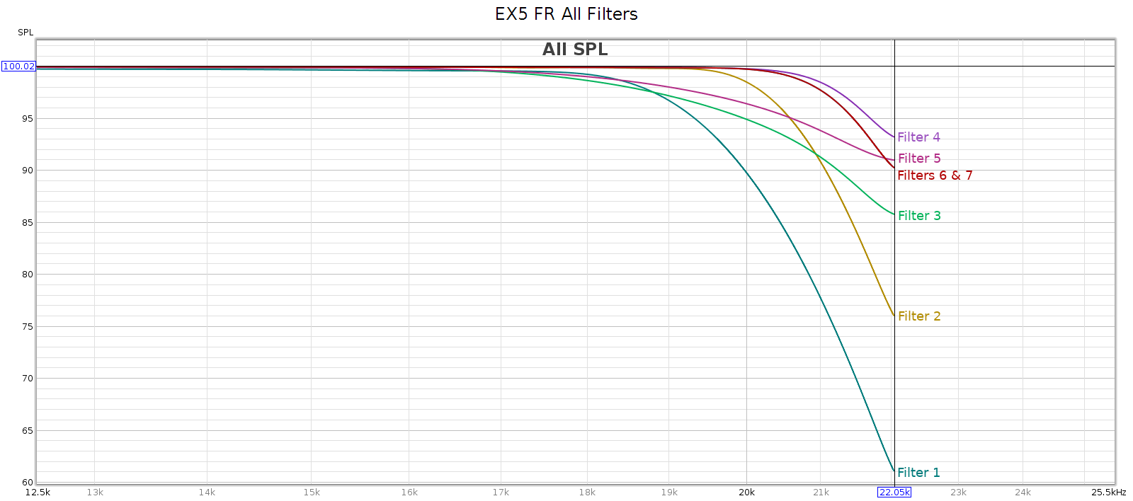
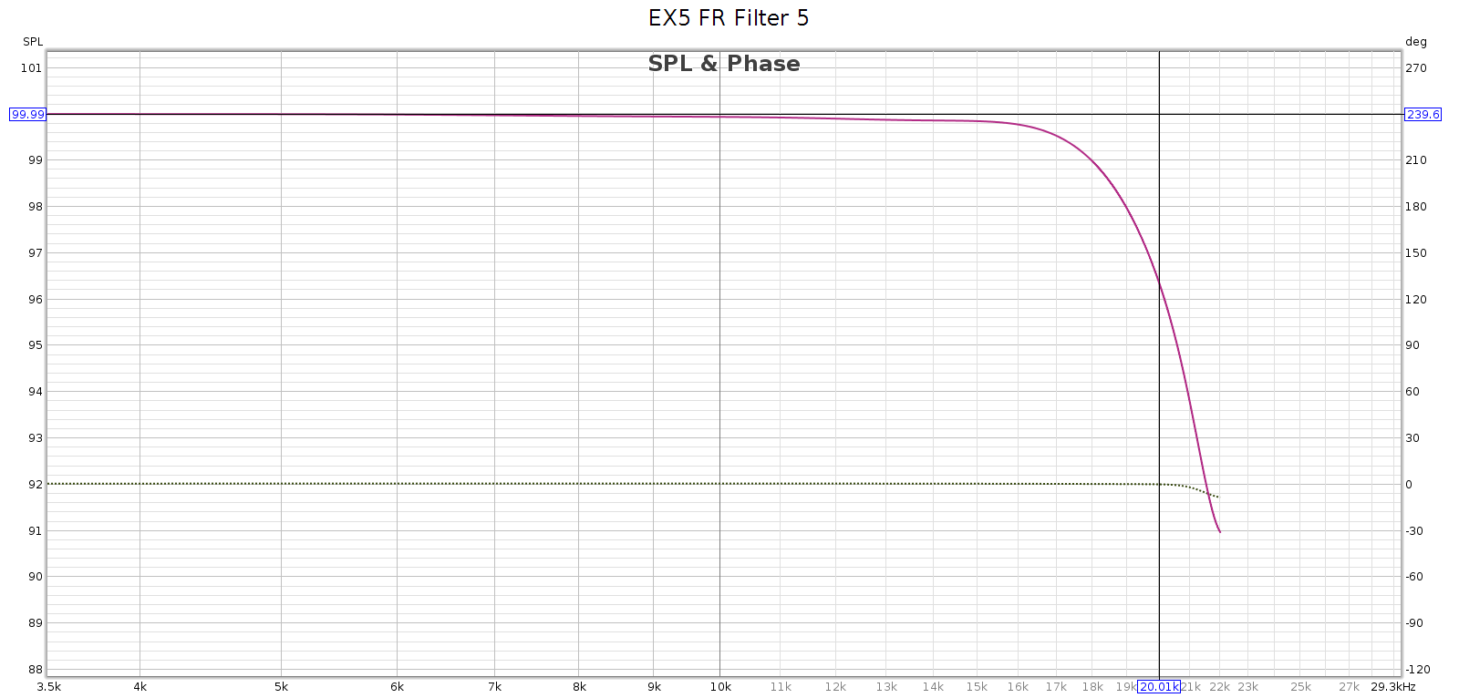
Here’s the frequency response of the EX5 digital filters at 44.1 kHz sampling:

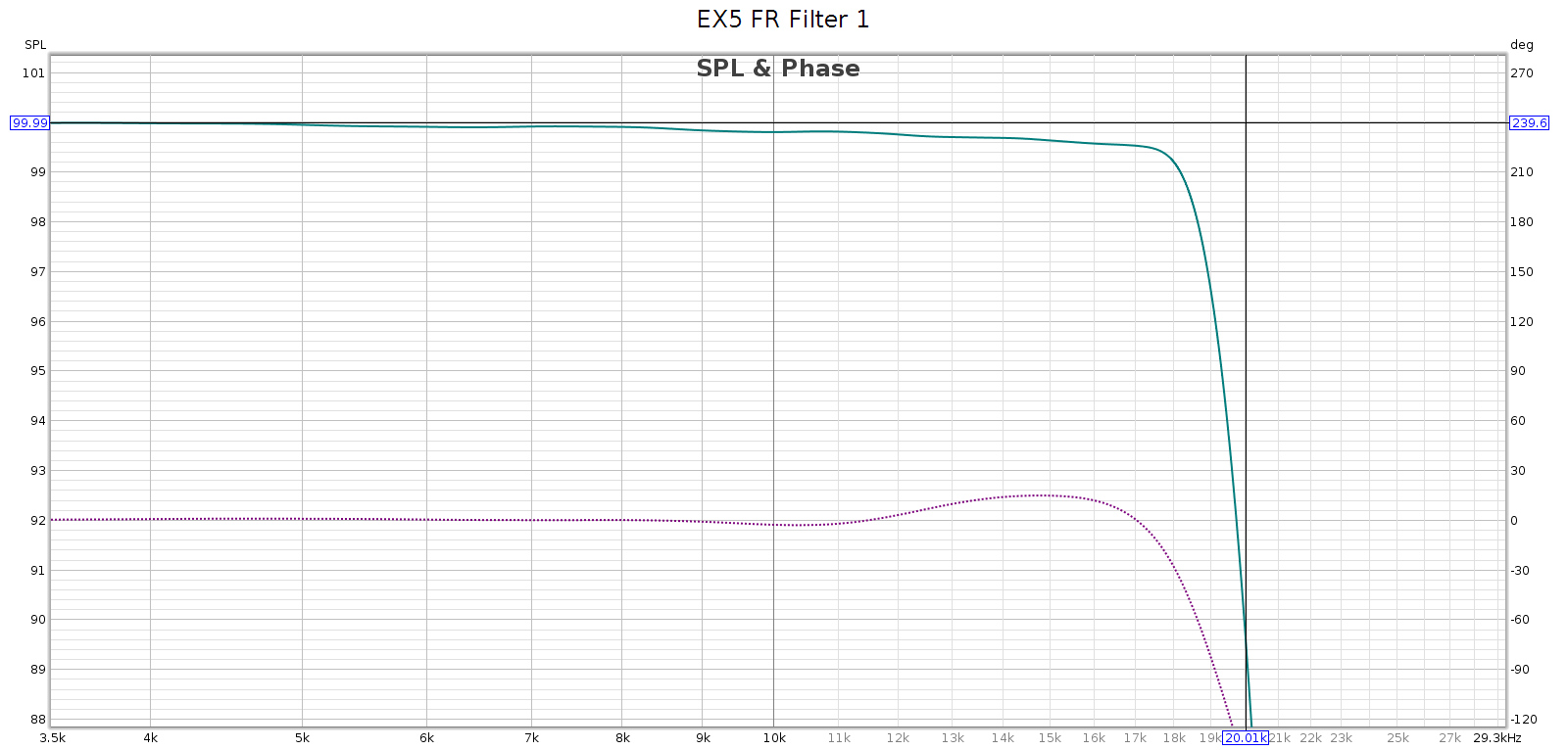
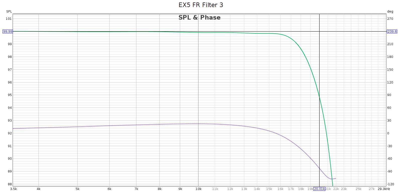
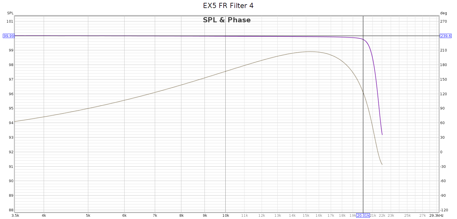
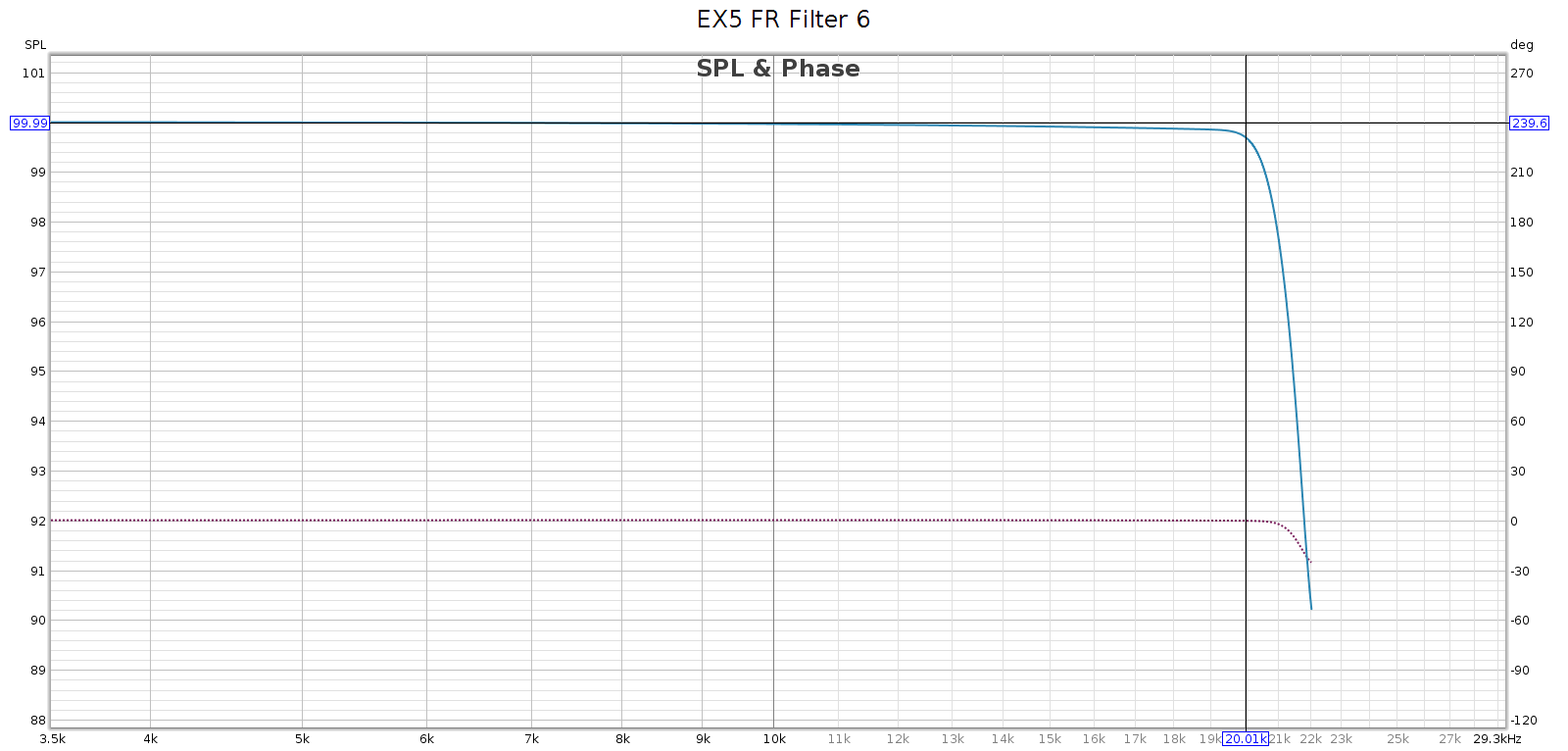
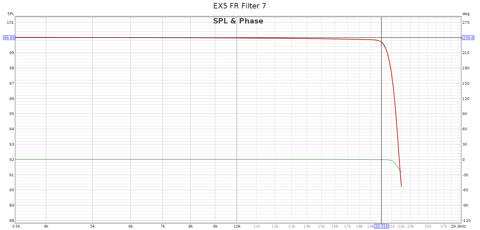
Filters 4, 6 and 7 are a bit lazy and don’t fully attenuate until 24.1 kHz. This is incorrect, yet benign.
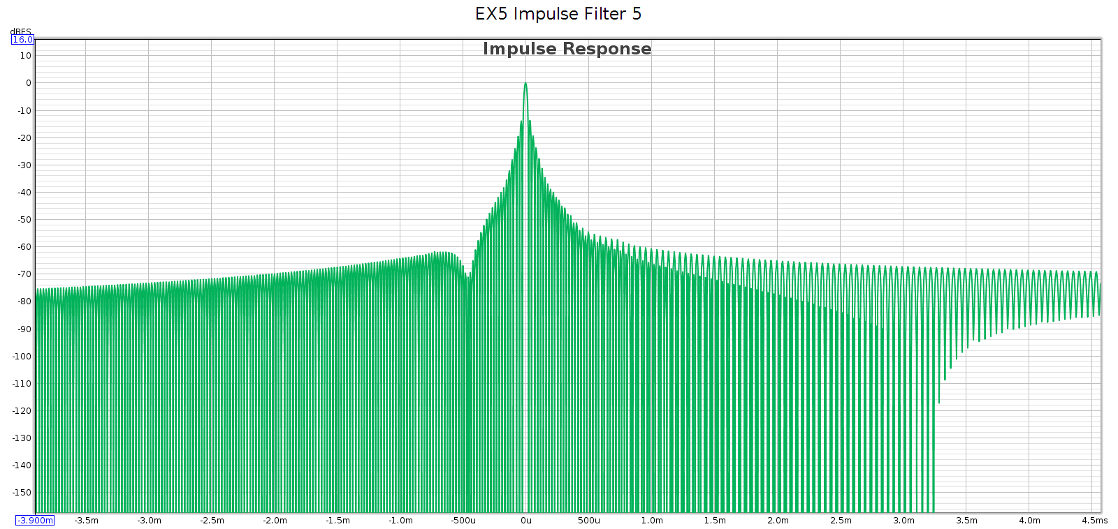
Filters 3 and 5 are very lazy and don’t fully attenuate until 28 kHz. This can be a problem.
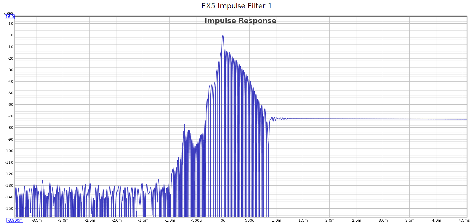
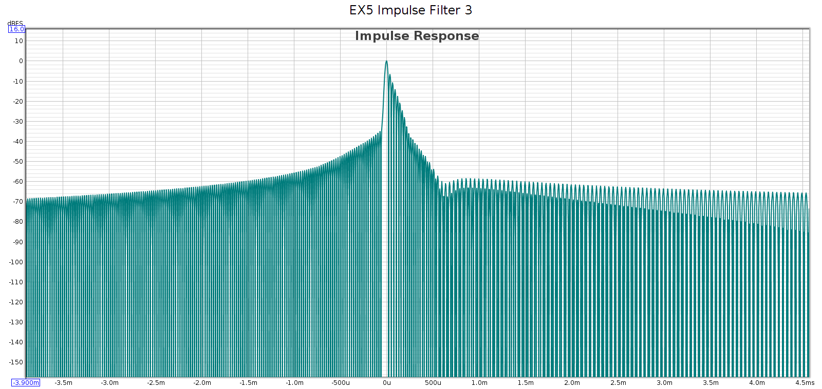
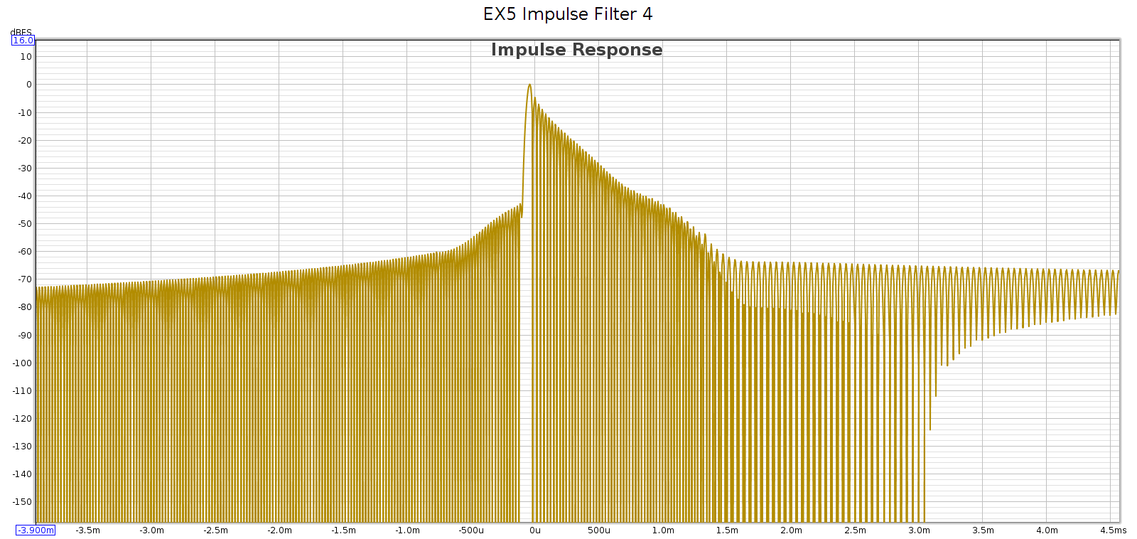
Filters 1, 3 and 4 are minimum phase.
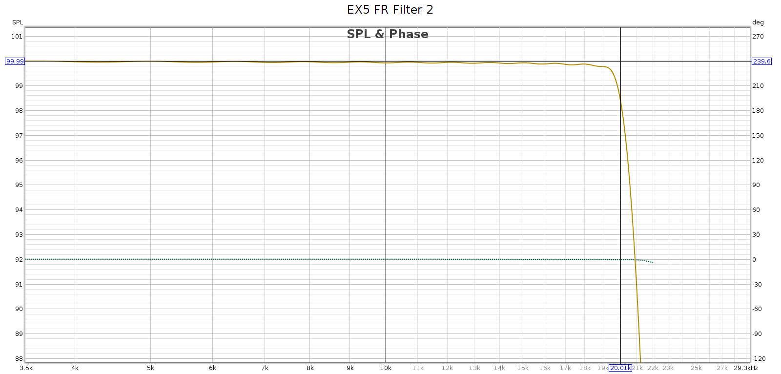
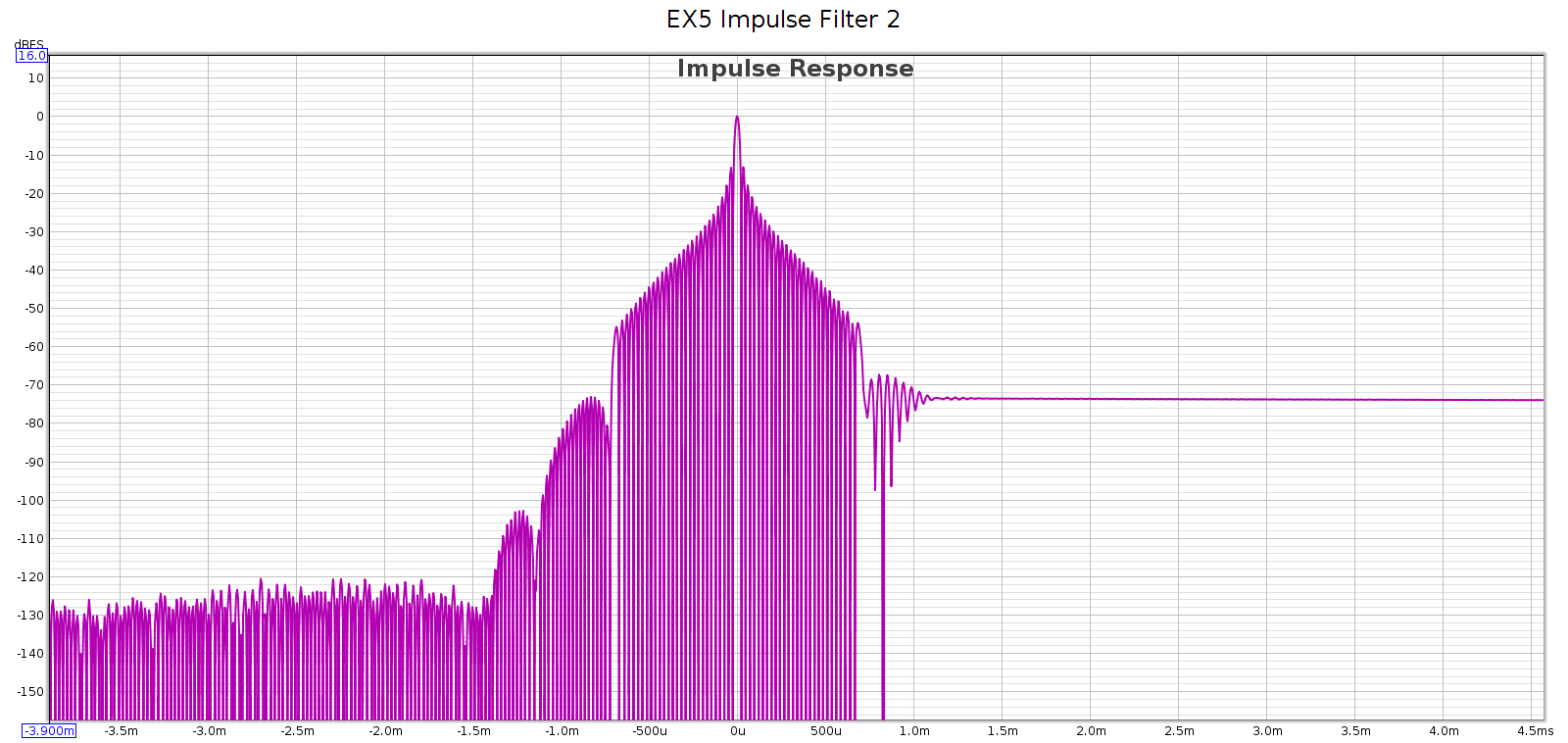
Filters 2, 5, 6, 7 are linear phase.
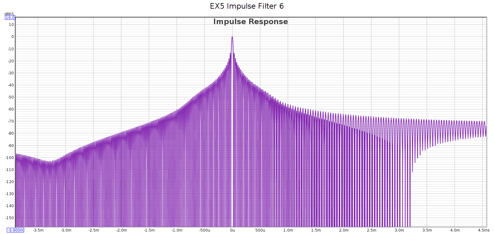
Filters 6 and 7 are identical in my measurements (both response & phase).

In summary:

  • Filter 2 is the most correct, but it is not perfect
    • Fully attenuated by Nyquist (surprisingly rare, but welcome)
    • Linear phase (flat phase vs. frequency)
    • It has a bit of ripple, not perfectly smooth
    • It has just a tad of passband attenuation: -1.5 dB @ 20 kHz
  • Filter 6/7 is as good as #2, with different tradeoffs
    • Fully attenuated by 24.1 kHz, thus any aliasing is above 20 kHz
    • Linear phase (flat phase vs. frequency)
    • No ripple – perfectly smooth response
    • No passband attenuation: -0.3 @ 20 kHz
  • Filter 4 is the best minimum phase filter
    • Fully attenuated by 24.1 kHz, thus any aliasing is above 20 kHz
    • Phase rises smoothly to +210* at 15 kHz, then drops to 0* at 21 kHz.
    • No ripple – perfectly smooth response
    • No passband attenuation: -0.2 @ 20 kHz

Put in reverse, why not use the other filters?

  • Filter #1 has significant passband attenuation: -10 dB @ 20 kHz
  • Filters #3 and #5 don’t attenuate until 28 kHz, thus leak high frequencies that can alias down to 16 kHz

How is the manual wrong? It gets 6 of the 7 filter descriptions wrong.

  • It labels #1 as fast rolloff apodizing, which is wrong
    • It rolls off slowly with significant passband attenuation, -10 dB @ 20 kHz
  • It labels #2 as slow rolloff minimum, which is wrong
    • It rolls of sharply with almost no passband attenuation
    • It is linear phase, not minimum phase
  • It labels #3 as fast rolloff minimum, which is wrong
    • It rolls off slowly with significant passband attenuation: -5 dB @ 20 kHz
  • It labels #4 as slow rolloff linear, which is wrong
    • It rolls off sharply with no passband attenuation
    • It is minimum phase, not linear phase
  • It labels #5 as fast rolloff linear, which is wrong
    • It rolls off slowly with significant passband attenuation: -3.6 dB @ 20 kHz
    • It does not fully attenuate until 28 kHz
  • It labels #6 as brick-wall, which is correct!
    • It has no passband attenuation, fully attenuates by 24.1 kHz, and is linear phase
  • It labels #7 as fast rolloff corrected minimum, which is wrong
    • This filter is identical to #6, and is linear phase

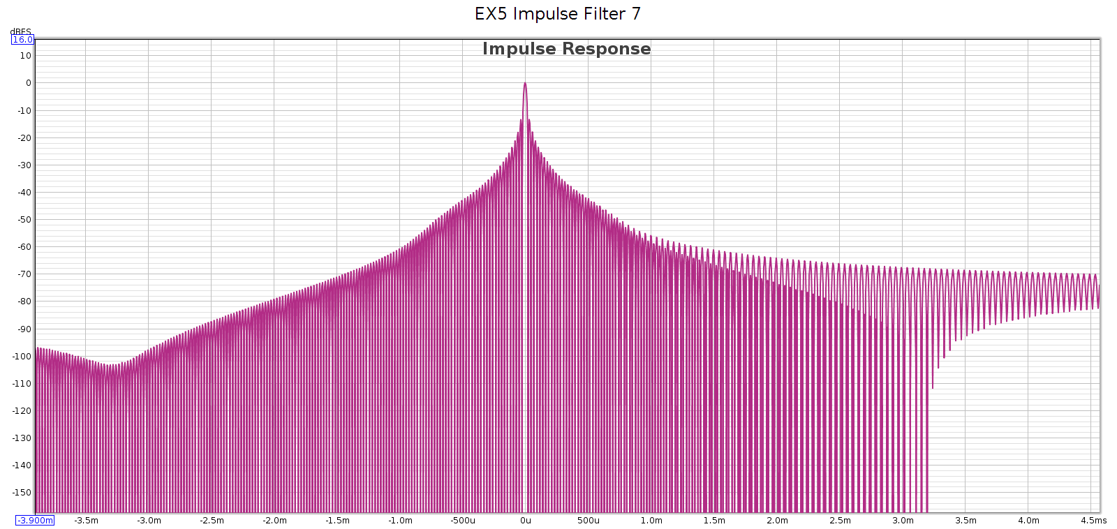
Measured at 44.1 kHz, here are the frequency response, phase, and impulse response of each of these filters. In each graph, the cursor marks the flat response corner @ 20 kHz. Below, note that the minimum phase filters have non-flat phase and asymmetric impulse response.

Filter 1

Filter 2

Filter 3

Filter 4

Filter 5

Filter 6

Filter 7

Comparison

The EX5 is such a great little device I couldn’t resist comparing it with my Corda Soul.

Frequency Response

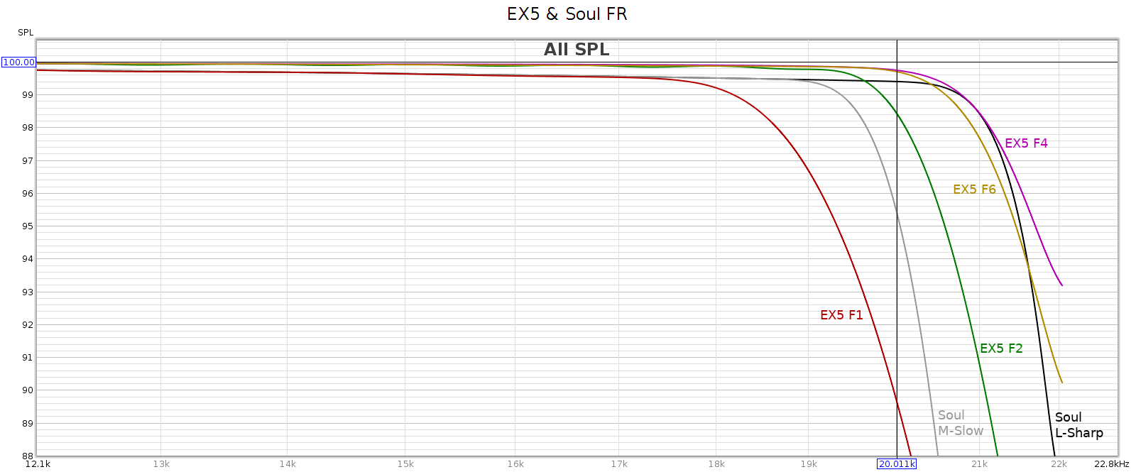
The Soul has 2 user-selectable filters. Here’s how they compare with the EX5:

The Soul’s linear phase filter (L-Sharp) is the best shown. It is the flattest in the passband, perfectly smooth with no ripples, and fully attenuates by 24.1 kHz faster than EX5 #6.

The Soul’s minimum phase filter (M-Slow) is between the EX5 #1 and #4.


Audio Review & Measurements: Denon DRM540 Cassette Tape Deck

Introduction

Years ago, I owned and used a Denon DRM-740, one of their best cassette tape decks. It was about as transparent as a tape deck can be (not very) and I recorded a lot of material on it. Recently I bought this piece of retro 1990s audio gear on eBay as a little blast from the past. I was curious if I could restore it to its original specs and performance.

Description

The DRM-540 is a standard 2 head cassette tape deck with electronic transport controls, Dolby B and C, HX Pro, and fine bias adjustment. You can Google it for details.

This unit arrived with a dirty, scratched heavily used exterior. Cosmetically, I’d rate it 2 of 5. This belied its interior condition. The heads looked fresh, no scratches or grooves. The inside was clean and all the service adjustment pots turned smoothly. Mechanically, it worked.

Restoration

The first thing I did was physically clean the heads, capstan and rest of the tape area with Q-Tips and isopropyl alcohol. It had years of oxidation and gunk. Next, I demagnetized the heads and metal transport parts. Now it was ready to play tapes. I connected the deck’s input & output to my PC sound card (an ESI Juli@).

First: speed adjustment. I played my calibration tape, which has 3 kHz on side A, 8 kHz on side B. The deck ran about 2% slow. That’s WAY off. I opened the top to get access to the motor speed adjustment screw. For coarse adjustment, I played the 3 kHz tone and listened with my phone and Spectroid app. It was quick & easy to get it within 1%. Then I recorded tape playback with Audacity and did an FFT / Spectrum Analysis. Back and forth a few times. Eventually I got the speed within 0.3%. That’s about as close as I could get, given the resolution of the adjustment screw.

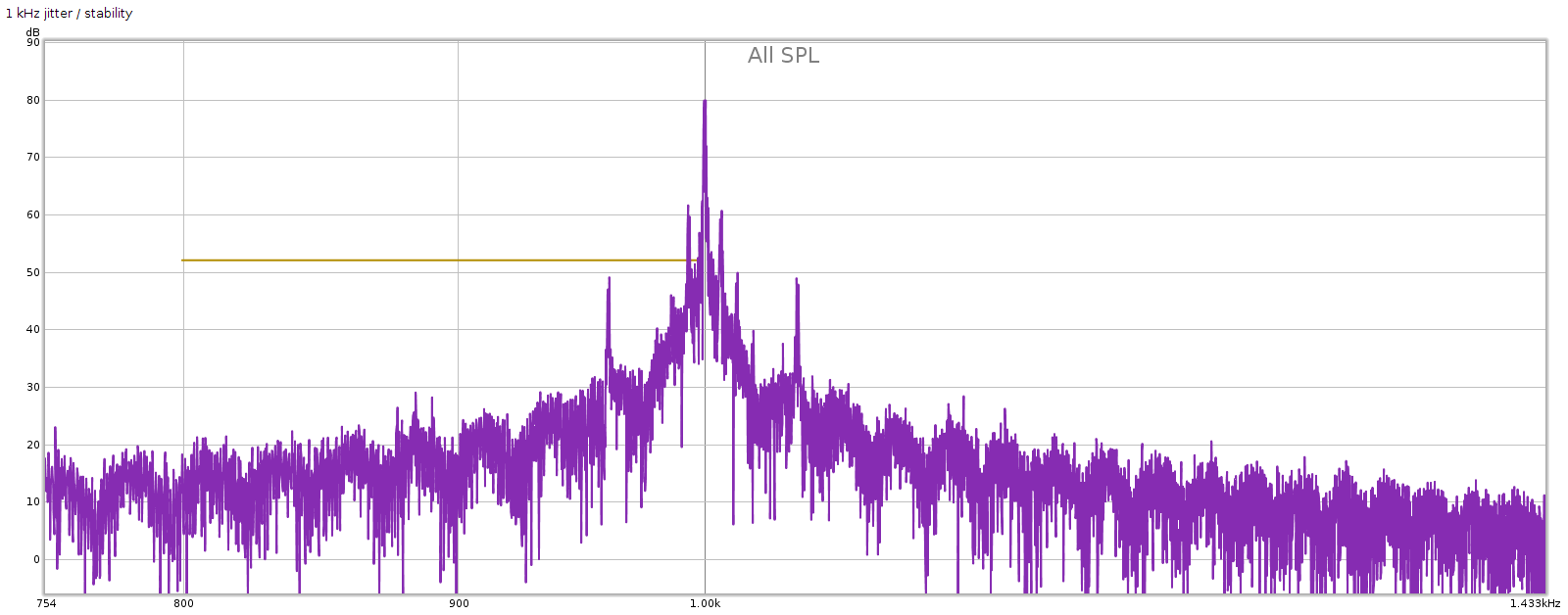
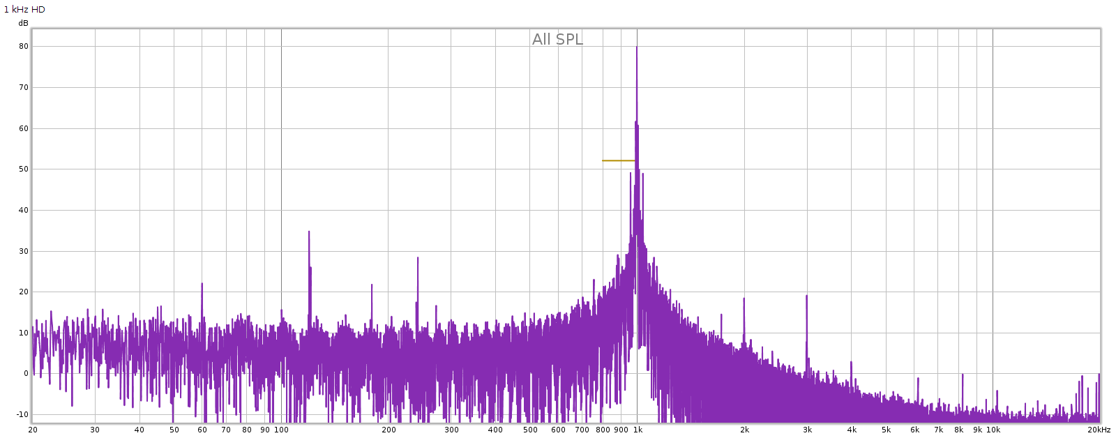
Here’s a closeup of the spectrum playing a 1 kHz tone. You can see sidebands near the center frequency, which show the frequency stability is imperfect. If this were a DAC we’d call that jitter:

Here’s the full spectrum for that same tone. You can see the 2nd & 3rd distortion harmonics are just under -60 dB. Not bad for a cassette tape deck.

You might notice that harmonic distortion from this tone is lower than the power supply harmonics at 60, 120, 180 and 240 Hz. It looks like this deck could be improved by better filtering the power supply. The power supply doesn’t appear faulty, it’s just that there’s no reason to spend a fortune making a super clean power supply, since the device will be limited by cassette tape performance.

Next: azimuth adjustment. This is a screw next to the playback head that changes the angle of the head to align it with the tape as perfectly as possible. I don’t have a scope, so I played the 8 kHz tone into the sound card while recording in Audacity. Slowly turned the screw back & forth to maximize the output level, until the screw was in the middle of the range of maximum output. This changes the channel balance, so I turned those internal pots to equalize them, then readjusted the azimuth. I went back and forth a few times until it was as close as I could get. The azimuth ended up in a very different position from where it started, so it was quite a bit off.

Then I went back to 3 kHz and adjusted the internal playback gain pots to equalize the channel balance, then to 8 kHz, which had slightly different balance. Back and forth a few times to minimize and equalize the difference.

Next: recording. I played REW frequency sweeps on the PC and recorded them. I used BASF Reference Maxima II tape, one of the best back in the old days. The L-R channels weren’t equal when recording, so I adjusted the internal recording gain pots to equalize them.

Dolby B is ubiquitous, so that is what I used for all the following measurements.

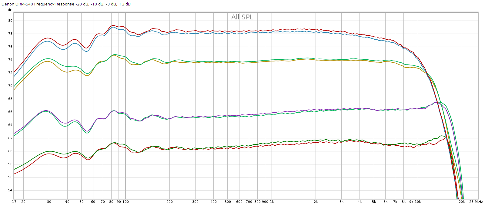
Here’s the frequency response measured at different recording levels: -20, -10, -3 and +3 dB. As expected the best (most linear) frequency response is at -20 dB, which is why that is the level used for its specifications. Frequency response tapers as we increase the level, yet it does so smoothly.

This deck meets or exceeds its specification, which is 20 Hz to 18 kHz, +/- 3 dB at -20 dB.

Next: bench testing: frequency response, distortion, SNR. I used the deck to record and play back the REW frequency sweeps and analyze them in REW. I did this at different settings: no Dolby, Dolby B and Dolby C. And I also did this while turning the external user-settable fine bias control to see whether it worked and how much impact it had.

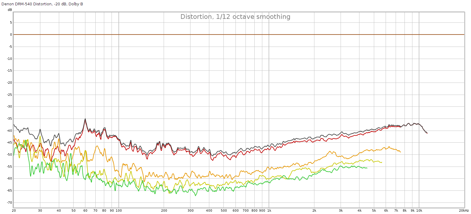
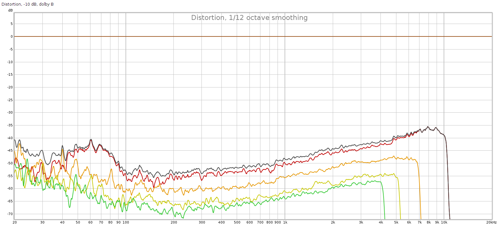
Here are some distortion graphs made at different recording levels. This is measured after recording and playback, so it includes total distortion from the deck itself, and from the tape used for recording. Thus it overstates the deck’s distortion and represents real-world results.

Distortion at -20 dB

Distortion at -10 dB

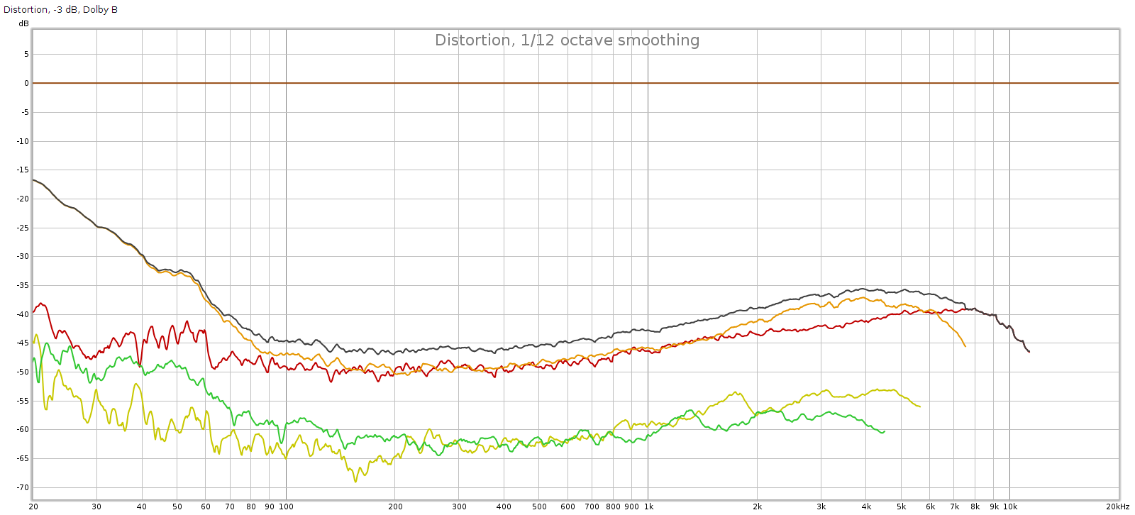
Distortion at -3 dB

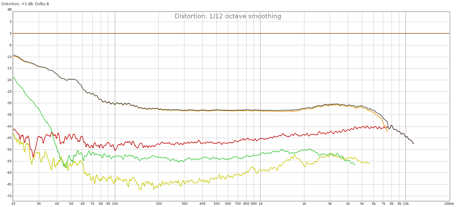
Distortion at +3 dB

Above, we see what we’d expect from a new deck. Distortion rises at high at high levels due to saturation, and it rises at low levels due to noise. The sweet spot for lowest distortion is around -10 dB recording level.

Another problem this deck had was that the recording level lights didn’t match between recording and playback. That is, record something with the levels just reaching 0 dB but when you play it back the lights indicate higher (or lower). I fixed this by adjusting the internal input and output level pots. Now the lights match between recording & playback.

Also, the drive motor developed an occasional squeak. I used a syringe to apply a tiny amount of low viscosity oil to the motor driveshaft/bearing interfaces. This eliminated the squeak. Then I had to readjust the speed again.

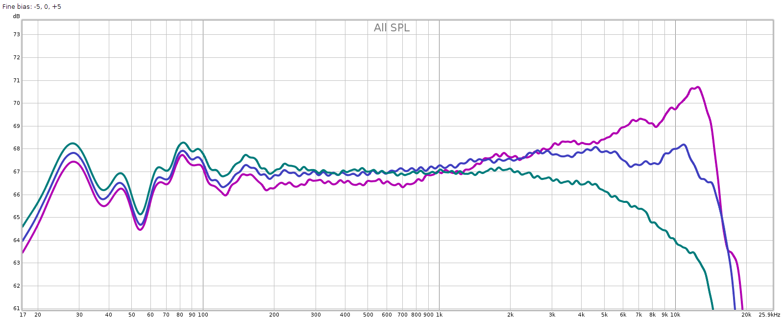
This deck has a fine bias knob on the front panel. The reason for this is that different types and brands of cassette tapes have different frequency response, so this enables you to fine tune the frequency response to each individual tape. I tested the effect of this knob, results below. Note that the graph uses 1 dB per division, so the frequency response is flatter than it looks.

The blue line is with the fine bias knob in its center position.
The magenta line is with the fine bias knob turned full left, CCW, the -5 position.
The green line is with the fine bias knob turned full right, CW, the +5 position.

The above graph shows that fine bias is like a tone control that tilts the frequency response like a see-saw whose center pivot is around 1 kHz.

Summary

Results: to my surprise, the deck performed on par with the specs from the manual.

  • Frequency response: 20 Hz to 18 kHz, +1 / – 3 dB
  • Distortion (with Dolby B)
    • At level -10 dB, THD at -50 to -55 dB (0.25%), with 2nd & 3rd harmonics at -60 dB
    • At level +3 dB, THD at -30 dB / 3%
  • Fine bias: -4 to +2 dB @ 10 kHz

Remember this is with a 20 year old blank tape that had been recorded on a few times. If anything, it understates the actual performance.

Finally, I did some subjective testing. Recorded a clean 96-24 digital album (Diana Krall & Tony Bennett), played it back and compared with the original. The differences are audible, but not as obvious as one would expect, given this vintage equipment and cassette tape limitations. It actually sounds pretty decent.

The original: http://mclements.net/audio/clip1-orig.flac
Recording: http://mclements.net/audio/clip1-rec.flac

The original is a high-res download resampled to 44-16 in Audacity.
The recording is the high-res download, played through my sound card, recorded on the DRM-540 in Dolby B with BASF Reference Maxima II tape, played back on the DRM-540 to the sound card’s analog inputs and recorded at 44-16.

Conclusion

Cassette tape is the vintage sound of the 1980s. It’s nowhere near as good and transparent as the modern digital equipment we have. We are so spoiled today! But, it’s not as terrible as its reputation and can sound pretty decent especially for casual listening, when the deck is clean and calibrated. And it was fun and educational to calibrate this deck, measure it and see the improvements.

Review: JDS Labs Subjective 3 Equalizer Kit

Summary

No Jedi’s training is complete until he constructs his own light saber. Audiophiles can benefit from this advice, as building audio gear is fun and educational, and improves our understanding and appreciation of this hobby. When it comes to building I’m very much an amateur, but I have some experience, having designed & built a passive attenuator and constructed a phono head amp in years past.

JDS Labs has a simple 3-band EQ they call the Subjective 3; they sell it as a product, and as a kit. The kit saves you $20 and gives you the fun & satisfaction of building it yourself. I couldn’t resist. Here’s a review.

My System

My desktop audio system is decent but not SOTA. My desktop PC (Ubuntu 18) is the player; it has an ESI Juli@ sound card, whose coax digital output goes to an SMSL SU-6 DAC, whose analog output goes to a JDS Atom amp. I listen on my 20+ year old Sennheiser HD580s, sometimes on Audeze LCD-2F.

Why not use DSP EQ like PulseEffects? I do in fact use this software. But sometimes I am capturing the audio stream to a file and want a bit-perfect copy without PulseEffects messing with it (resampling, applying DSP). And while the PulseEffects multi band parametric EQ is a precision tool for accommodating the response to rooms and headphones, sometimes all you need to do is tame an overly bright or dull recording, in which case a simple old fashioned 2 or 3 knob equalizer is simpler & easier to use.

JDS Subjective 3 Kit

I ordered the kit and it arrived in 2 days (that was the cheapest shipping available). JDS says it is simple and a good first kit for those who want to dip their toe in the DIY water. I agree with this assessment, with caveats that I’ll mention below.

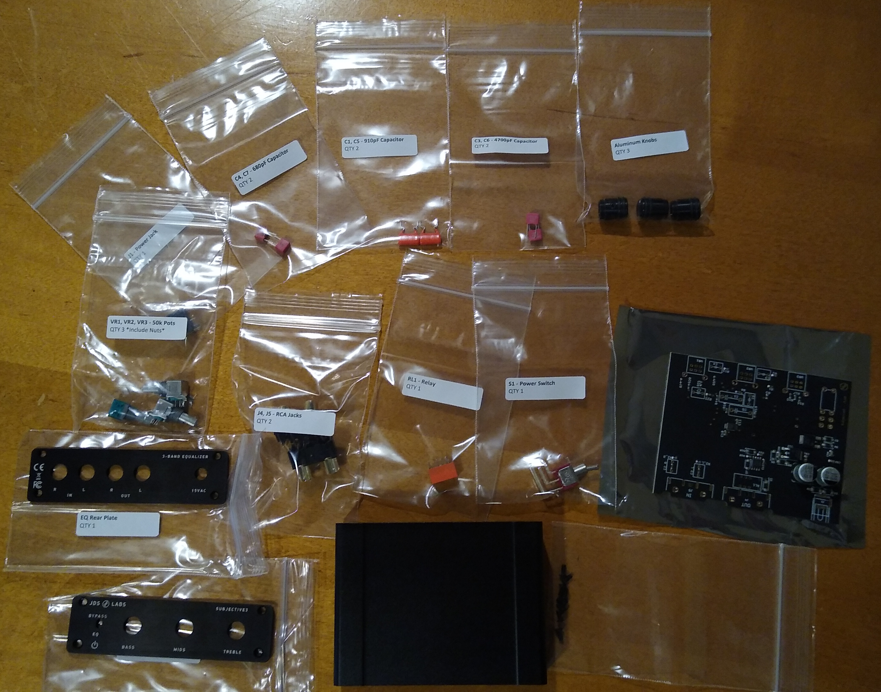
Here’s how the kit arrives:It includes all parts including the power supply (not shown), and the parts are of high quality: Alps RK09 potentiometers, Vishay and WIMA capacitors.

Installing the Parts
Soldering

Assembly is straight-forward. The instructions simply say, “insert all capacitors, solder and trim”. This may sound daunting for noobs, but each part is bagged with a part number that is also printed on the circuit board where it plugs in. Find each number on the board and plug in the corresponding part.

The key here is to use a soldering iron with a very fine tip and relatively low power (12 W). Avoid cold solder joints. That is, heat up the parts to be joined until the solder melts when touching those parts — not the soldering iron tip itself. Use just enough solder to sink and seep through the hole, but not so much that it makes a glob.

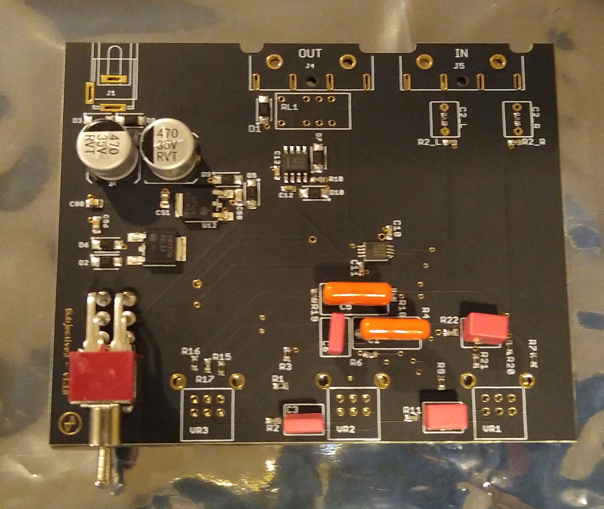
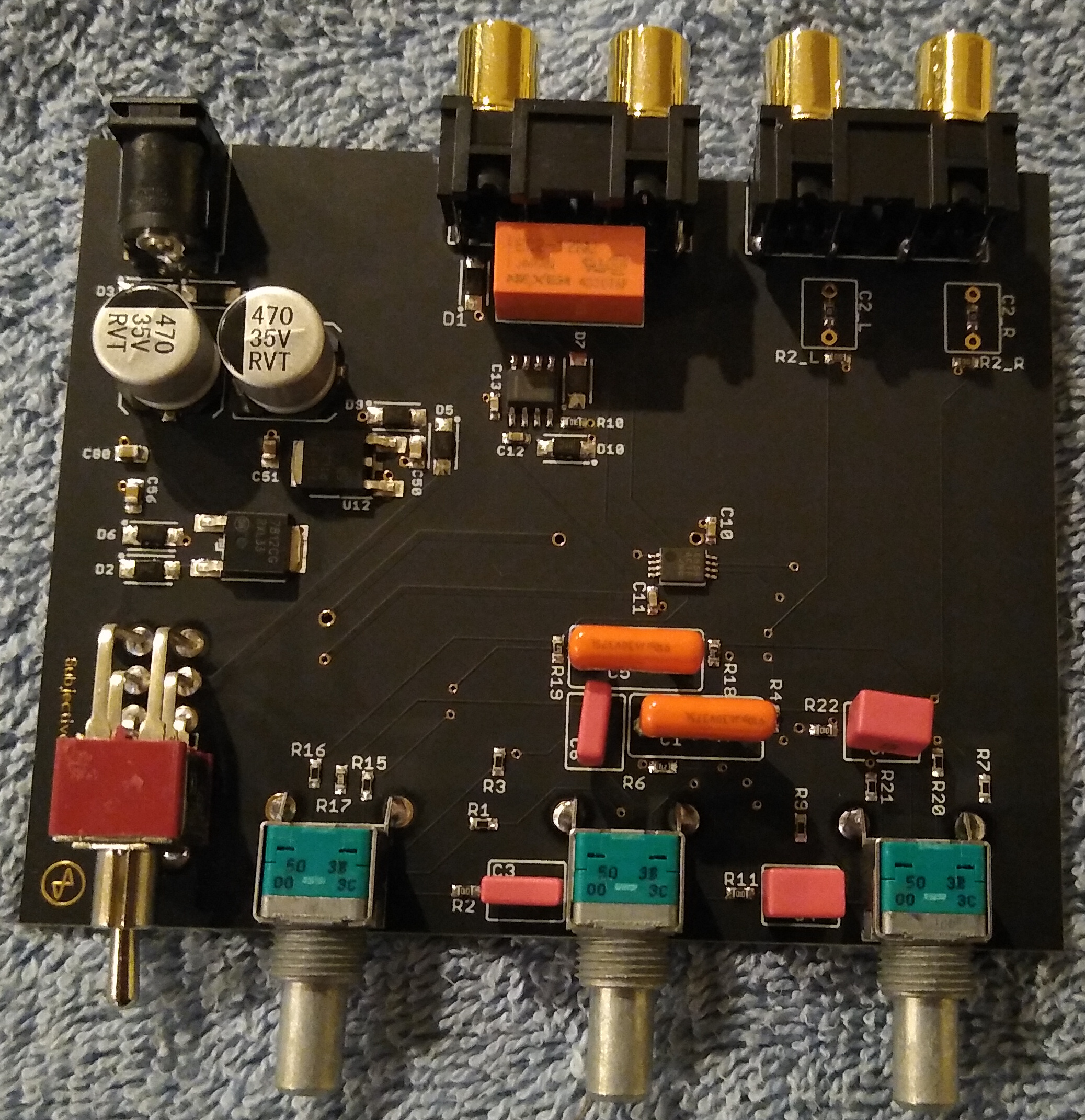
Here’s what it looks like after installing the capacitors and power switch:

Position and Fit

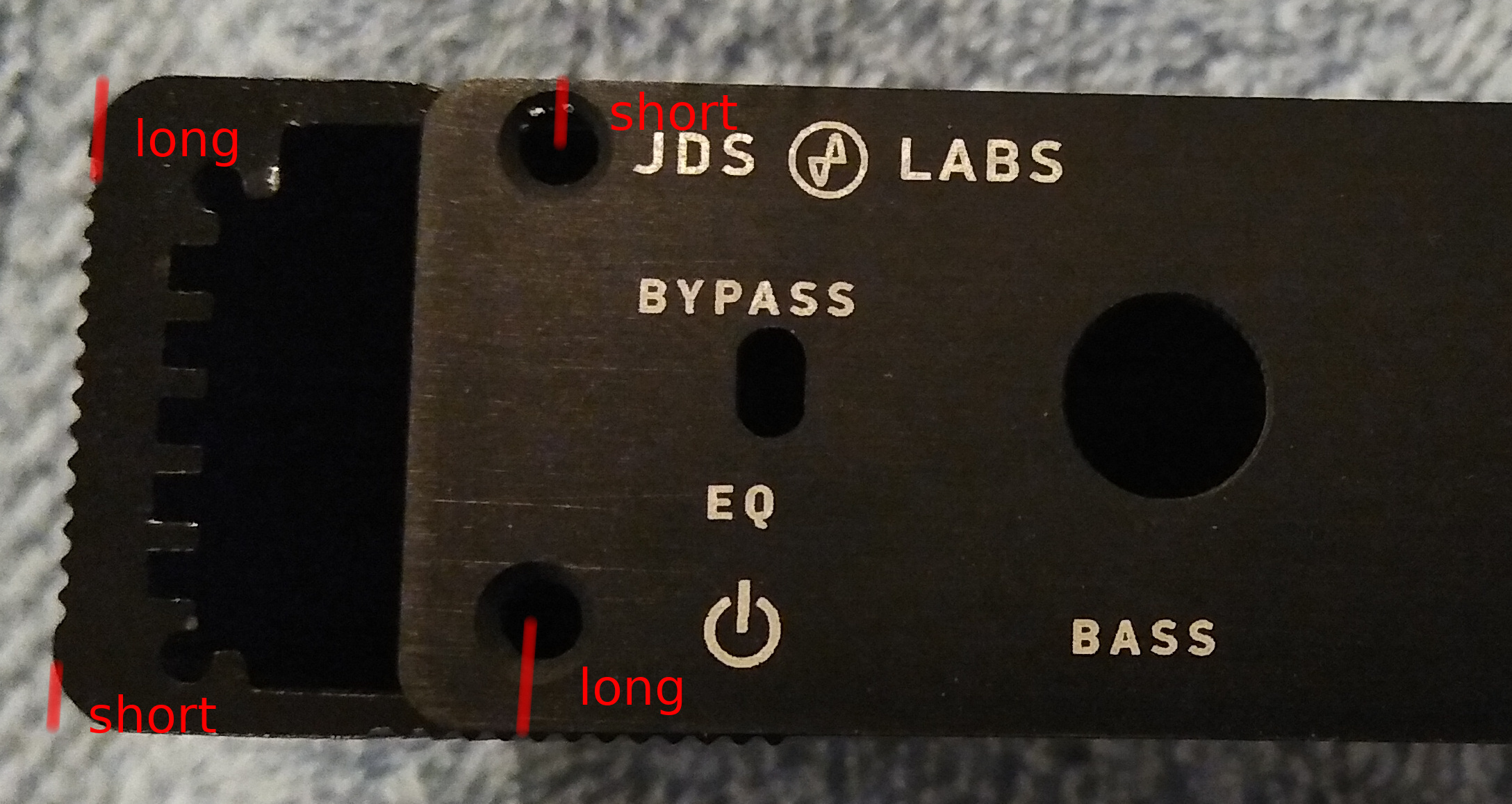
Some of the parts soldered to the board must match holes in the case when assembled: knobs and switches. If they ride too high or low on the board, the case won’t fit. When I was checking this alignment, I noticed that the case is asymmetric. It looks symmetric at a glance and the asymmetry is subtle, so this would be worth mentioning in the instructions. A picture’s worth 1,000 words, and I reversed the faceplate and case to highlight the difference:

At first, I didn’t notice this and when I checked alignment, it looked like I needed to solder the power switch and potentiometers in a position slightly above resting flat on the board, in order for them to line up with the holes in the case. But it turns out this is not necessary. Solder them flat to the board and use the faceplate as your clue that the “long” distance is the bottom of the case.

Installation: Complete

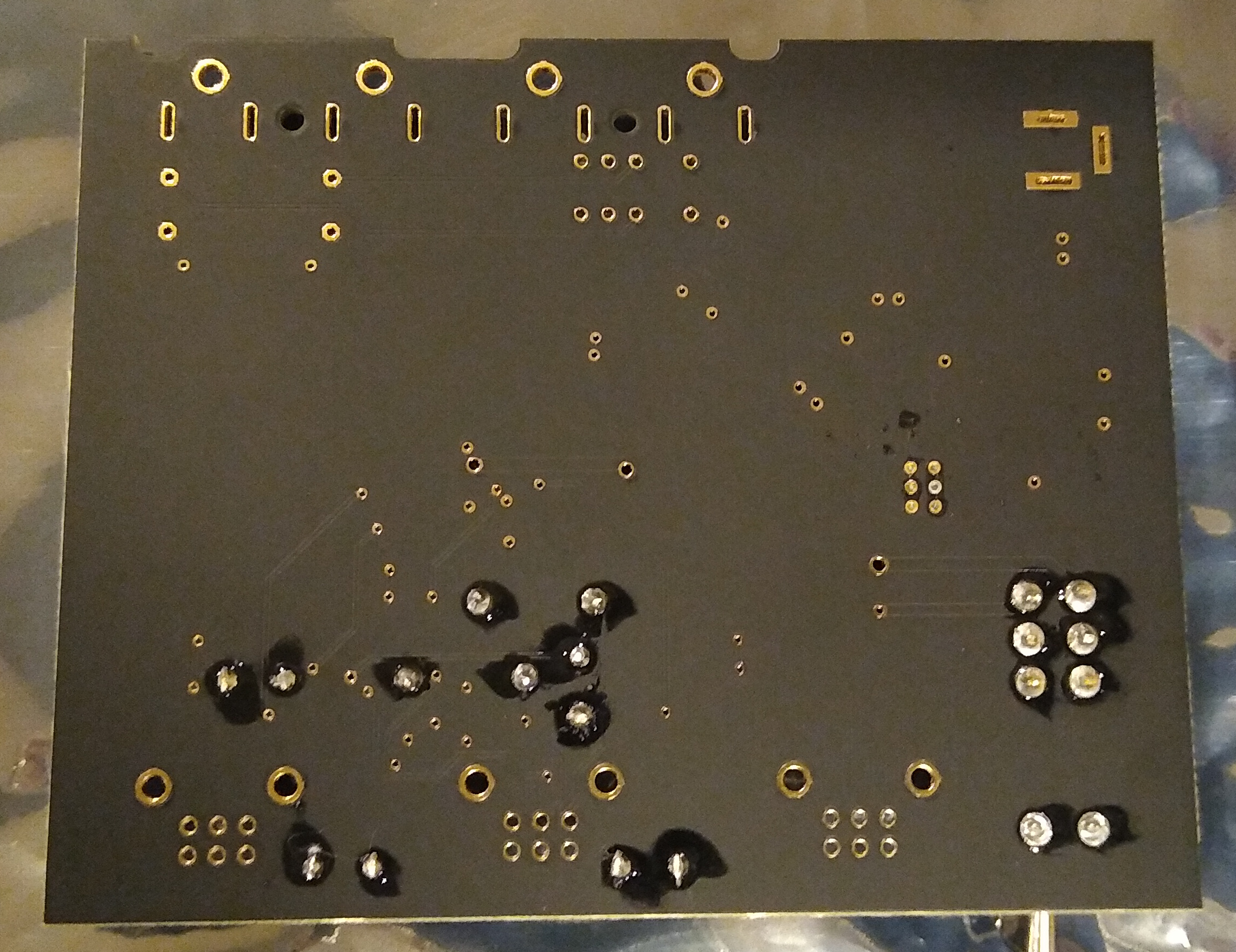
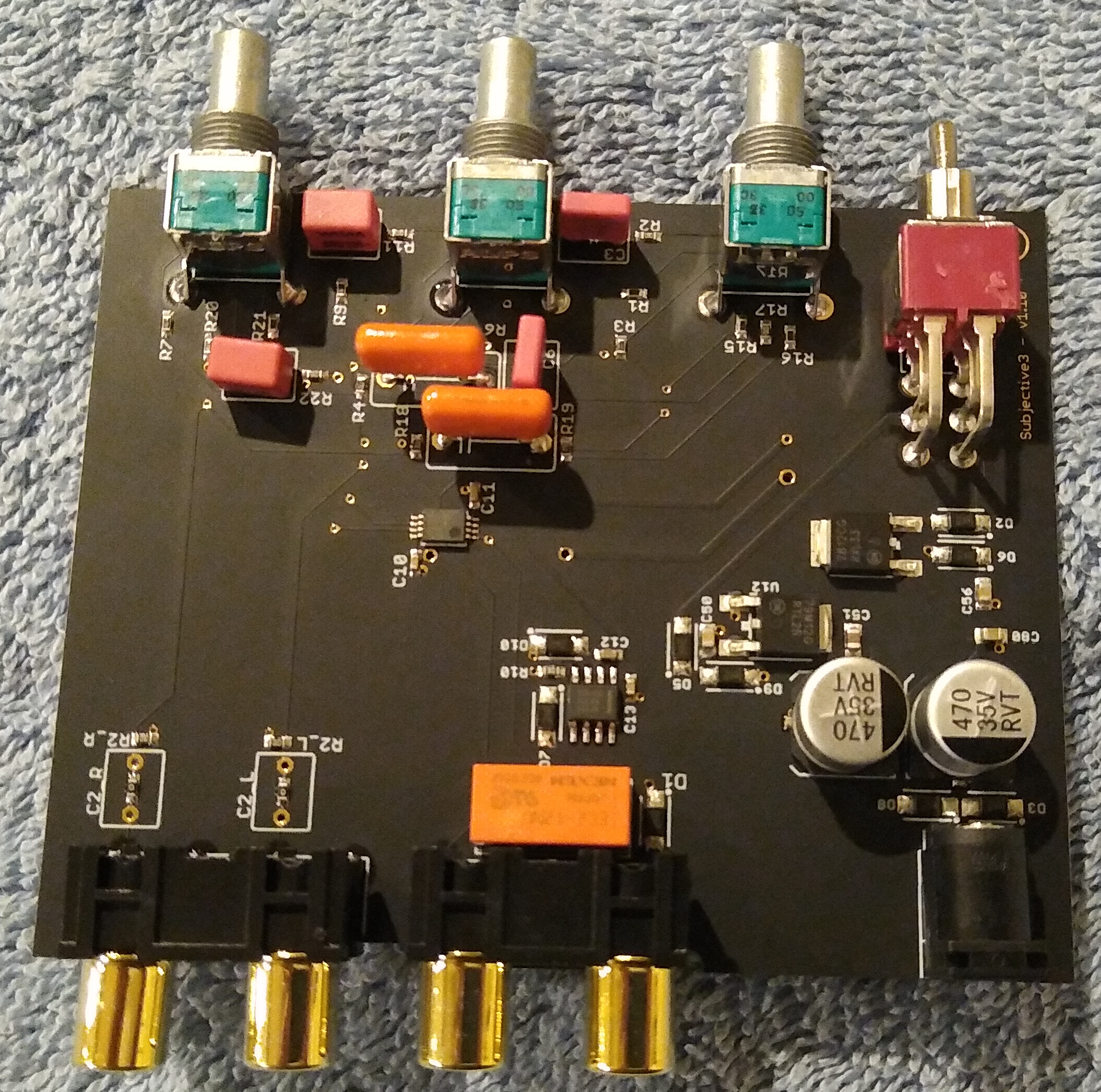
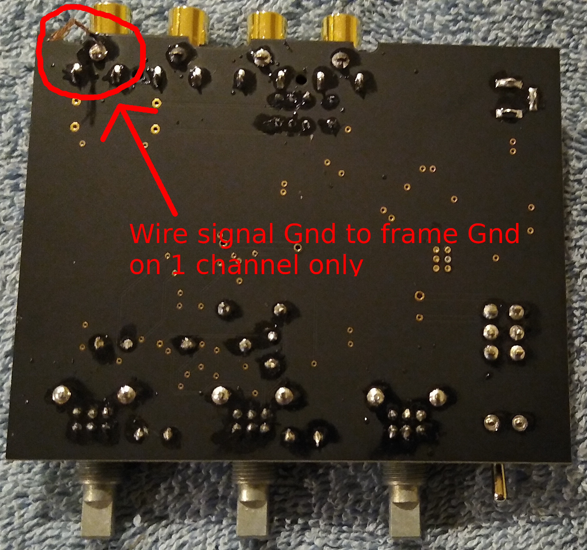
Here’s the board with installation complete: two views of the top and one of the bottom:

The above photo shows 2 important things: fine soldering, and grounding.

Fine Soldering

Each potentiometer has 8 contacts, 6 of which are in a tight grid. Soldering these can be tricky for those wielding an iron for the first time. Start with the middle contacts and work your way outward. Hold the iron near vertical so it doesn’t accidentally contact other stuff on the board. Be careful to use just enough solder to fill the hole without forming a glob that could touch the nearby pins.

Grounding

In the above left you can see that one (but not both) of the signal grounds is wired to the frame. This is something I discovered years ago through trial & error troubleshooting pesky ground loops when I was building a passive attenuator, and also on a phono head amp that I built. If neither signal ground is connected to frame, you can get a ground loop causing a “hum”. Also, if both are connected to frame. But if only 1 is connected to frame and the other is not, it helps break ground loops.

Assembly: Complete

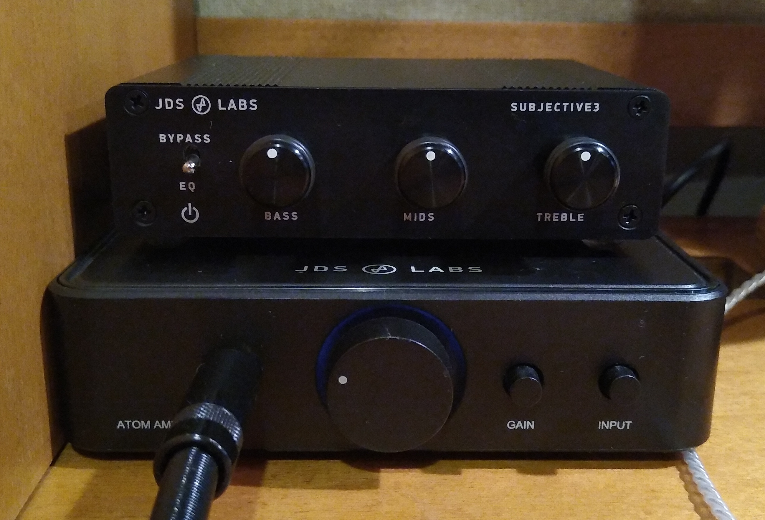
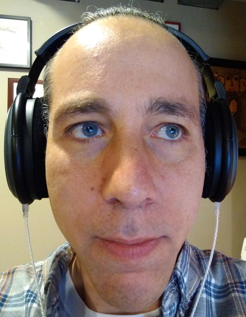
Here’s what the completed kit looks like up close, with my JDS Atom amp:It’s quite small, even smaller than the JDS Atom which itself is a small amp. Here’s what it looks like with the headphones (you can see the wooden headphone stand I made years ago):

Listening

I powered it up, no smoke — great! I played some music with the tone knobs in the center detent, switching back and forth between “EQ” and “Bypass”. There should be no difference in the sound. Indeed they were almost identical. But there seemed to be a very slight difference. In Bypass mode I heard just a hint of “grain” or “edge”, especially in the upper mids / lower treble where our hearing perception is most sensitive. This was the opposite of my expectation, which was that if there was any difference at all, bypass mode would be more transparent. I was playing a very high quality recording of 5 voice ensemble, which highlights midrange purity, revealing distortion quite well.

Our hearing perception is not reliable enough to trust, but it’s not wrong often enough to ignore. So I put the EQ in a loop with my Juli@ card and used REW to take some measurements. Maybe I’m just hearing things, it’s not really there. Or maybe I made a mistake in the build. Either way, measurements would give a helpful baseline.

Measurements
Baseline

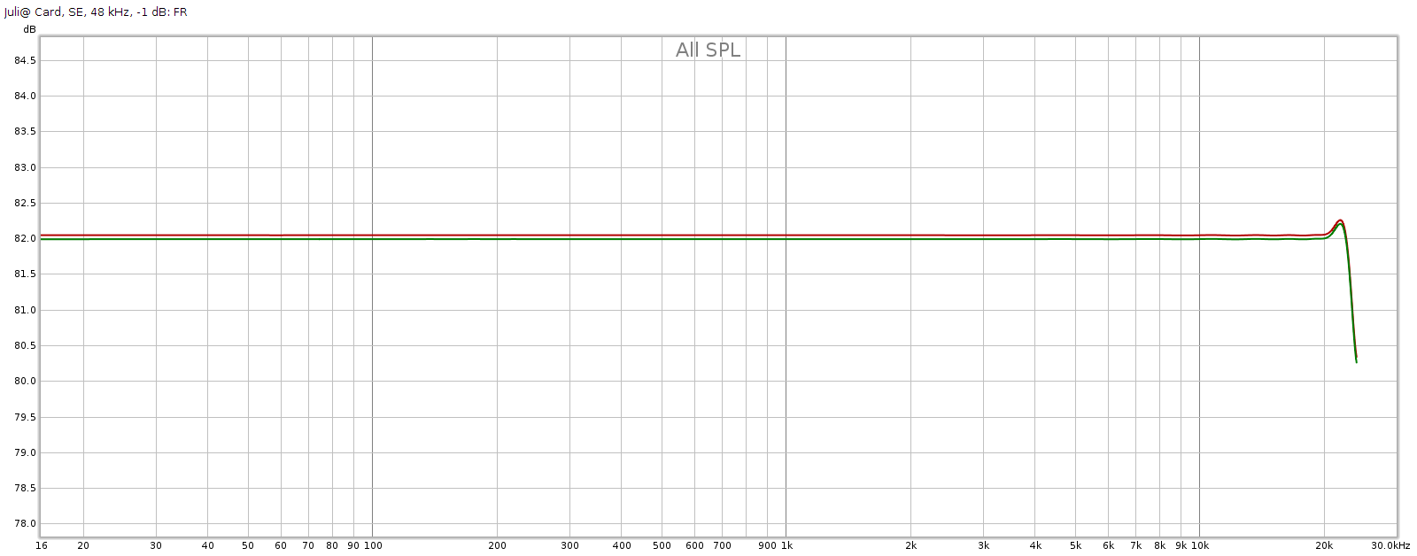
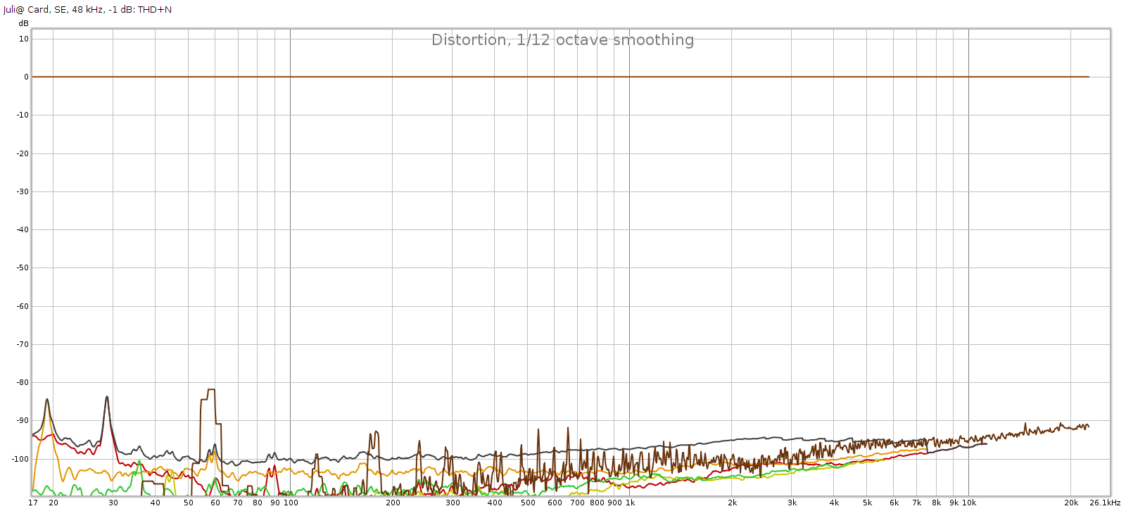
My Juli@ card is the baseline and it is not perfect, so let’s look at its FR and distortion. I played 48 kHz sweeps in REW at digital -1 dB for this:Frequency response is flat with << 0.1 dB variation. The bump above 20 kHz seems to be an REW anomaly. It has a slight channel imbalance which at < 0.05 dB is immaterial. Distortion and noise are mostly -90 to -100 dB, which is the limit for 16-bit.

Subjective 3 EQ: Bypass

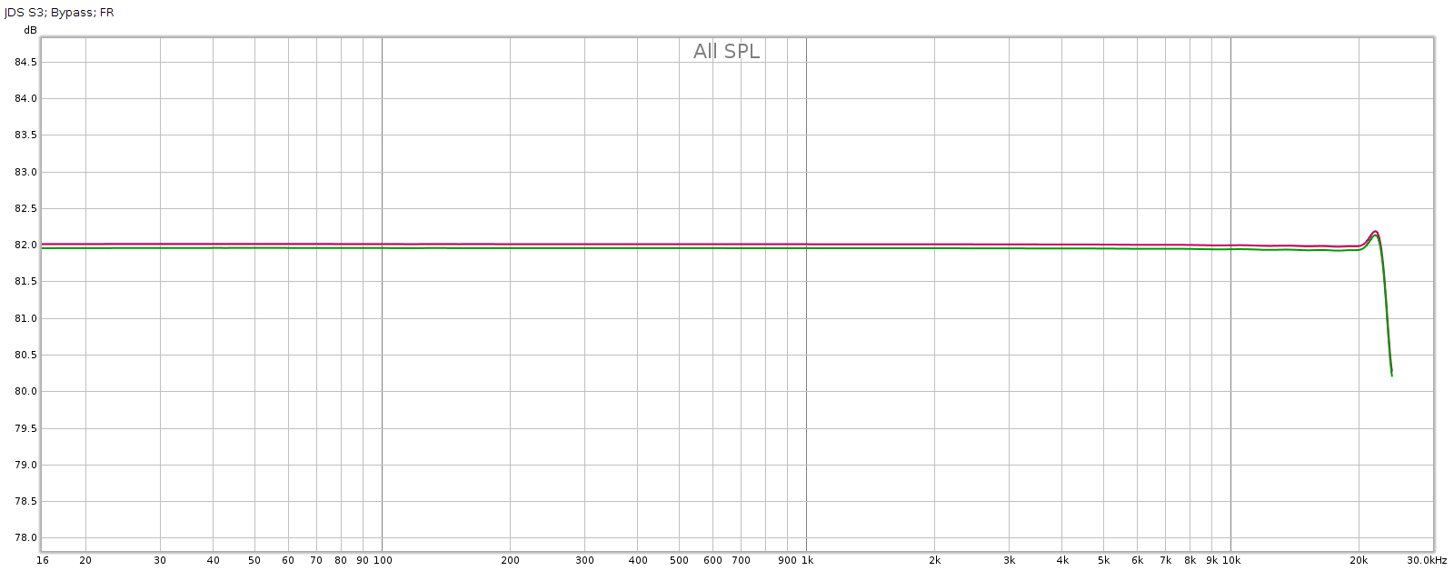
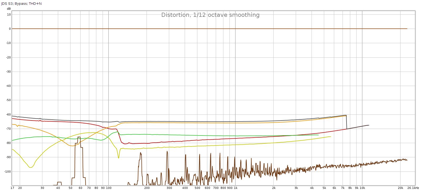
Against this baseline, let’s see what the Subjective 3 looks like. First, bypass mode:Frequency response is perfect, no difference from the loopback. But we have quite a bit of distortion and noise! At about -60 dB it is likely inaudible, but it is approaching thresholds where it might become audible under ideal worst-case conditions.

Subjective 3 EQ: Frequency Response

Now let’s flip the switch the EQ mode with all the knobs in their center detents.

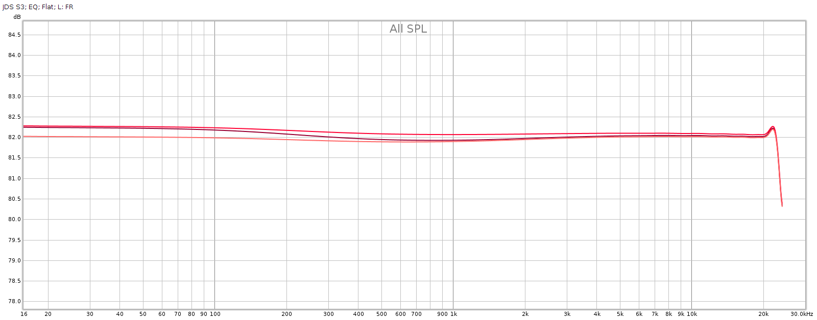
Here are 3 measurements of the L channel. In between measurements, I rotated each of the tone control knobs several times through its full range then re-centered it to the detent for the measurement. This reveals how consistent it is.

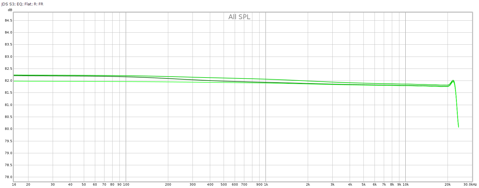
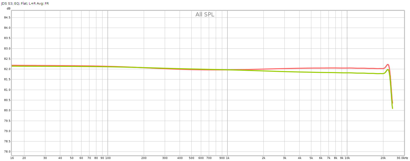
Note: the Y scale is 0.5 dB per division in order to reveal small differences. Red is left, Green is right, just like a boat or airplane.Here are 3 measurements of the R channel, taken the same way:Each shows variations around 0.25 dB. I’m pretty happy with that, it’s about as good as analog potentiometers get. These differences in consistency should be inaudible. Here are the average responses of each, shown together.Channel balance is essentially perfect below 2 kHz, at which point it gradually increases to a max of about 0.25 dB at 20 kHz with the L being slightly stronger.

So the consistency of the knobs, and the L-R channel balance, are each within about 0.25 dB.

Subjective 3 EQ: THD+Noise

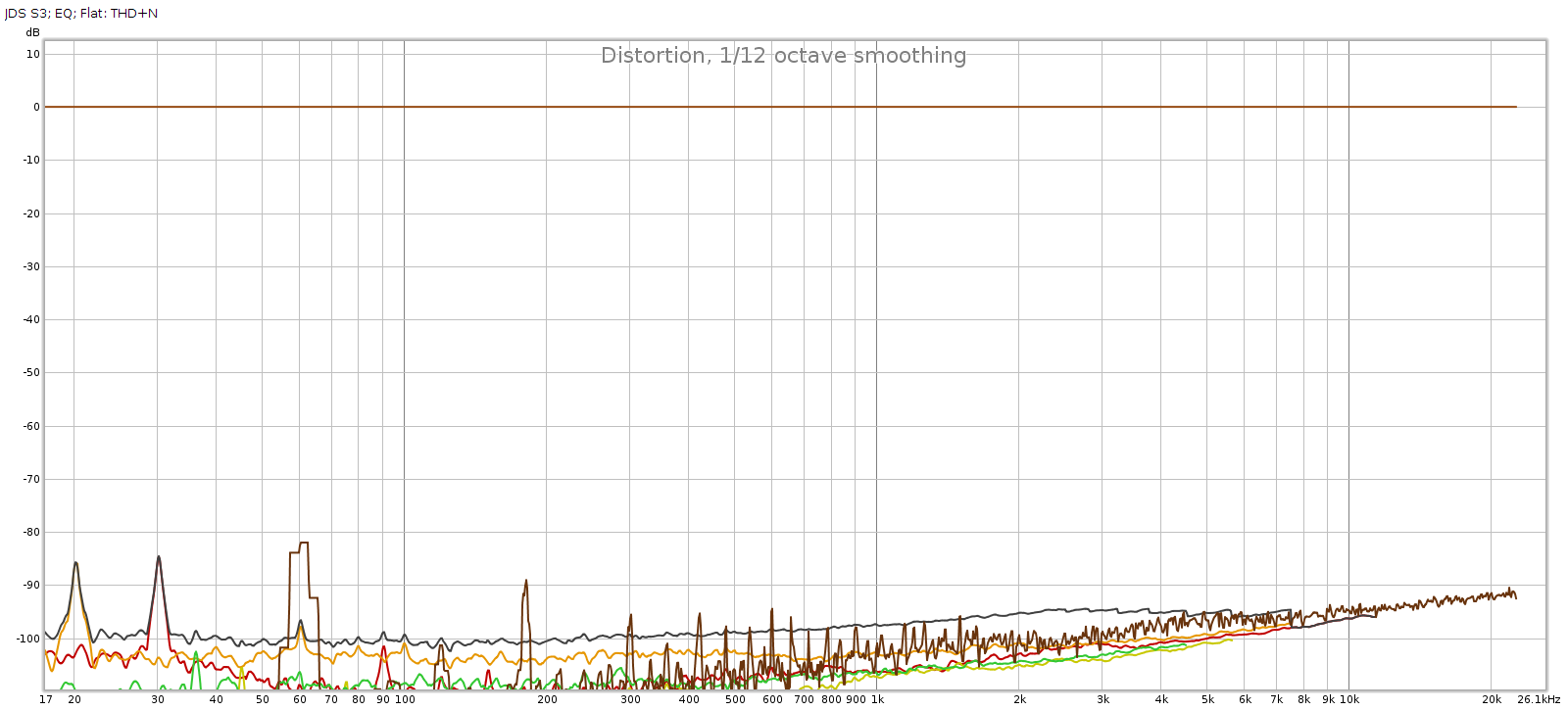
Now let’s see if that increased noise we measured in bypass mode, is also there with EQ enabled:Nope! That’s good news. In EQ mode, it doesn’t add any distortion or noise. Of course, no device is perfect. But whatever it does add is below the levels of my sound card and thus masked and inaudible. JDS Labs publishes a THD+N specification of .0022% which is about -93 dB. We have at least that here.

Subjective 3 EQ: Response Curves

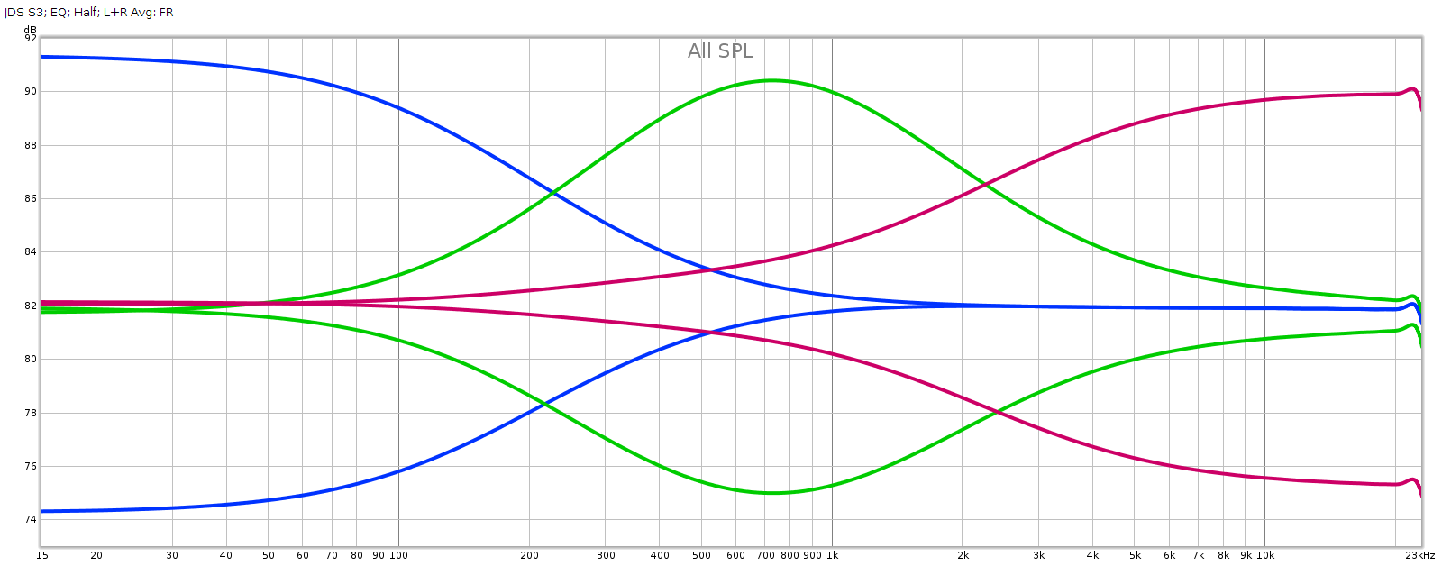
Now let’s see what the tone control knobs actually do to frequency response. I measured each knob at its half-way positions, negative and positive. This is approximate, as I can only eyeball the half-way position. So in the graph below, the curves + and – variations aren’t quite the same, but the important thing is the shape of the curve which shows the frequencies each of the knobs changes:

Obviously, blue is bass, green is midrange, and red is treble. And of course I had to zoom out the Y-axis, which is now 2 dB per division in order to keep the curves on-scale. These curves match nicely to the documentation.

Conclusion

The JDS Labs Subjective 3 EQ is a nice little kit. It is inexpensive, uses high quality parts and is easy to build with clear instructions. It sounds and measures clean and transparent in EQ mode. It has good consistency and channel balance. The knobs have a lot of range; just turning from 12:00 (center detent) only “1 hour” to 11:00 or 1:00 makes a noticeable difference. This makes the knobs quite sensitive and the full range is far more than I’ll ever use.

The only real drawback is that bypass mode introduces a fair bit of distortion. At -60 dB it’s close to thresholds of inaudibility, but may become perceptible on certain kinds of well engineered recordings on very high quality playback gear. That said, this issue is unique to bypass mode; the S3 EQ is consistent and clean enough to simply leave powered on in EQ mode all the time.

Note: I contacted JDS Labs in case the distortion in bypass mode was due to a mistake I made in building or measuring this device. They confirmed that it is known, and they’re revising the board to fix this. As I write this update it is Feb 2022 and they just sent me the revised board and parts so I can build another one. I’ll report back soon…

The problem is fixed. The S3 in standby mode now measures the same as a loopback connector, as it should. No more added distortion. In active mode (turned on) it is the same as before. JDS will be shipping this revised version soon.

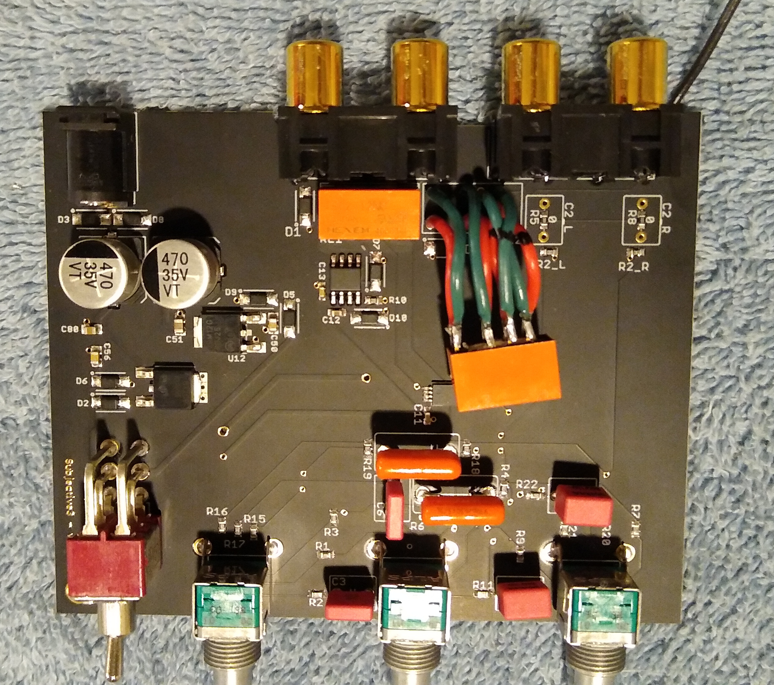
Here’s the new board. I couldn’t simply solder the 2nd relay into the board, because 2 pairs of pins had to be reversed. So I wired it individually in order to cross pins 4-5 and 8-9. That was tricky for someone with only moderate soldering skills like myself. In production boards, this relay can be soldered directly into the board just like the one next to it, much easier.

Headphones: HD580 vs. LCD-2F

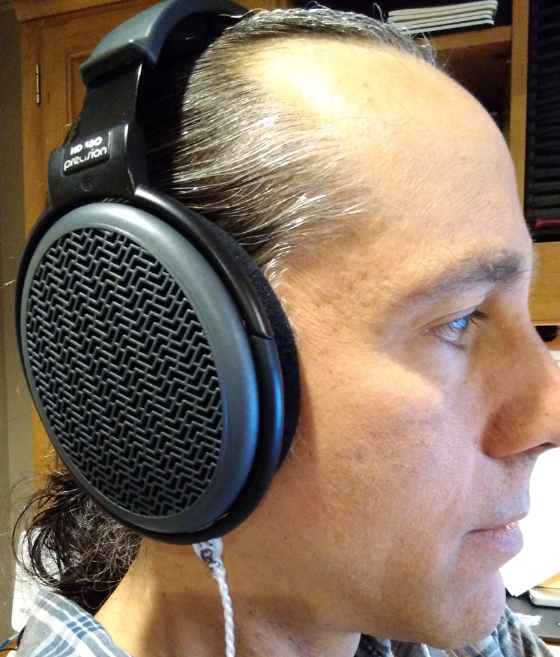
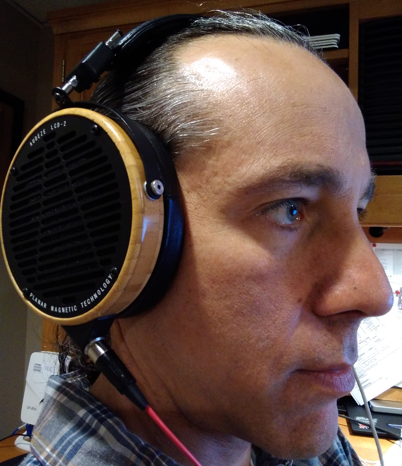
I’ve been listening to headphones for decades. Over the years I’ve tried many different ones. The Sennheiser HD580 and Audeze LCD-2F are my favorites. I own a pair of each and use them daily. This is a direct comparison.

Sennheiser HD580

I bought my pair in 1999. Over the years I’ve replaced the pads and cable several times, and kept the drivers clean. They still work like new.

They aren’t made anymore, but three models currently made are almost the same:

  • Sennheiser HD600
  • Massdrop 58x
  • Massdrop 6xx

Audeze LCD-2F (Fazor)

I bought mine in 2014 with the original Fazor drivers. Then in 2016 I sent it to Audeze to replace the drivers with the lastest/revised version.

Fit & Comfort

The HD580 are smaller, lighter, and better ventilated. They stay in place as I move my head around. I can wear them all day without any discomfort.

The LCD-2F are bigger, heavier, and less ventilated. They stay in place as long as my head is upright but if I bend my head forward & down, they try to fall off. They are comfortable, but after 2-3 hours the weight (especially on the headband) begins to drag.

In this category the HD580 wins.

Efficiency and Impedance

The HD580 are rated at 330 ohms, but their impedance ranges from 300 through most frequencies, rising to a peak of 600 ohms at 100 Hz. Voltage sensitivity is on the low side at 0.17 V for 90 dB SPL. A phone can’t drive them properly, you’ll need a headphone amp. And if that headphone amp (or phone) has a high output impedance, it will boost tones near the impedance peak (around 100 Hz) making the headphones sound warmer.

The LCD-2F are 70 ohms at all frequencies; being planar magnetic, their impedance vs. frequency curve is flat. Voltage sensitivity is a bit higher than the HD580 at 0.11 V for 90 dB SPL. They play 3-4 dB louder than the HD580 at the same volume setting (voltage). A phone can almost but not quite drive them properly, you’ll need a headphone amp. The frequency response of these headphones will not be affected by the amp’s (or phone’s) output impedance.

Overall, the LCD-2F are easier to drive than the HD580, and you may get acceptable results driving them from a phone, but you’ll need a headphone amp to get the most out of either.

Sound Quality

HD580

  • Bass: rolled off below 100 Hz
  • Midrange: smooth and linear
  • Treble: rolled off above 10 kHz
  • Distortion very low, but high (5%) in the bass
  • Voicing: a slight brassy/boxy coloration

LCD-2F

  • Bass: smooth and linear to subsonic
  • Midrange: smooth and linear
  • Treble: dip at 4 kHz
  • Distortion very low throughout (even in the bass)
  • Voicing: open, transparent uncolored

Summary

The LCD-2F has near-perfect ruler flat response from subsonic through the upper mids (to around 2 kHz). In the treble, it has the Audeze “house sound” with a dip around 4 kHz, though compared with the rest of the LCD models it has the smallest dip and is the most neutral. If you don’t EQ this dip, the sound is a bit soft — yet not dark, as the treble from 7 kHz on up is not attenuated.

The HD580 has a more linear, neutral response through the treble, though it rolls off both the lowest bass and the highest treble. The HD580 also needs EQ to lift the bass below 100 Hz, but when you do, the bass sounds wooly or soft as distortion becomes audible.

Overall, these are 2 of the best headphones money can buy in terms of sound quality. Of course you can spend a lot more, but you can’t really get much better sound. Without EQ, I prefer the HD580, yet with EQ, I prefer the LCD-2F.

That said, the differences are small enough that you need really good recordings and a quiet listening environment to hear it. And the HD580 is less expensive, more comfortable, and has less need of EQ. So it is the value king: 90% of the sound quality for 20% of the price.

Firefox and Audio Streaming

I use my desktop computer as an audio source for music listening. Listening to high quality (lossless) music over the browser, I’ve explored different browsers and how they deal with audio. This is on Ubuntu 18 Linux with Pulseaudio. I’ve set up the audio to avoid resampling as much as possible.

I tried about 10 different browsers on Ubuntu. Every one but Firefox resamples audio to some fixed rate, either 44.1 or 48 kbps. Firefox is the only one that passes audio through unmolested. Or, at least it used to. Primephonic is a classical music streaming service that passes audio uncompressed at whatever rate the albums were recorded (from 44.1 to 192 kHz).  I could listen to different albums and watch Pulseaudio change the sampling rate to match whatever rate each was recorded. At least until some time in Feb 2021, when Firefox’s behavior changed.

Here’s a summary of the changes:

Firefox now ignores the audio stream’s native rate and attempts to stream it at the highest rate the system will support. This means it will resample the audio rather than play it at its native rate.

If Pulseaudio’s avoid-resampling is set to true, then that rate will always be the highest rate the system supports. For example, with my Juli@ sound card it is 192 kHz. Otherwise (avoid-resampling set to false) that rate is the highest rate Pulseaudio is configured to use. That is either default-sample-rate or alternate-sample-rate, whichever is higher.

So in order to listen to music on Firefox without resampling, you must:

  • Set both of Pulseaudio’s rates to the native rate of the stream you are playing.
  • Set Pulseaudio avoid-resampling to false.

Essentially, you are forcing the system to play all audio at a single rate that exactly matches the audio you are playing.

And indeed, the irony is that in order to avoid resampling, you must set avoid-resampling to false!

Incidentally, why the irony? I can only speculate. Cubeb, the audio engine in Firefox, asks Pulseaudio what is its highest sampling rate. If Pulseaudio is avoiding resampling, then it reports its highest rate to be the highest rate the audio card supports. But if Pulseaudio is resampling, then it reports its highest rate as whatever rate it is resampling everything into. Seems logical. But it ironically leads the reverse of the intended behavior. The root of the problem is cubeb. It should pass audio to the system at its native rate, and let the system deal with it. Cubeb is being too smart by half, trying to deal with that itself.

High Res Audio on Ubuntu: Part 3

Once we’ve got it all set up, we want to test it while playing audio. It’s the only way to know for sure it is working as expected. To do this, we’ll be using the Linux Pulseaudio command-line tool pacmd.

If you jumped directly to this page, you may want to read part 1 and part 2.

Once you’ve tested your setup, possibly made adjustments, and confirmed they are working, you may want to read about streaming audio from a browser.

Basic Audio Device Info

To start, enter this command:

pacmd list-sinks

A “sink” is an audio output device. Even if you only have 1 sound card in your system, it may support multiple sinks. And you may have multiple cards. So you may see a lot of output here.

Let’s use grep to shrink the output to only the fields most useful to us:

pacmd list-sinks | grep -e 'sample spec:' -e 'channel' -e 'buffer' -e 'latency:' -e 'name:' -e 'alsa\.card'

On my system, it returns this:

name: <alsa_output.pci-0000_04_02.0.analog-stereo>
current latency: 0.00 ms
sample spec: s32le 2ch 176400Hz
channel map: front-left,front-right
fixed latency: 185.76 ms
alsa.card = "1"
alsa.card_name = "ESI Juli@"
device.buffering.buffer_size = "262144"
device.buffering.fragment_size = "70560"

This tells you I have an ESI Juli@ sound card that is currently set to 176.4 kHz sampling and 32-bit signed. My Pulseaudio configuration uses sample rates of 176400 and 192000, so this is the default sample rate. This is 4x oversampled for normal CD quality (44.1 kHz) and 4x oversampled for normal DVD quality (48 kHz).

Now I play an audio file that happens to be sampled at 96 kHz. While it’s playing I run the above command again and it returns this:

name: <alsa_output.pci-0000_04_02.0.analog-stereo>
current latency: 170.65 ms
sample spec: s32le 2ch 192000Hz
channel map: front-left,front-right
fixed latency: 185.76 ms
alsa.card = "1"
alsa.card_name = "ESI Juli@"
device.buffering.buffer_size = "262144"
device.buffering.fragment_size = "70560"

You can see that Pulseaudio has changed the sample rate to 192 kHz. Why? I have “avoid resampling” enabled, so it should play at the audio file’s native rate of 96 kHz. But Pulseaudio will never use a sample rate lower than what you configure. Since it can’t use 96 kHz, it uses the next best thing, which is an integer multiple of the native rate. That is why it switches to 192 kHz.

Resampling

The above command showed us the current state of the audio device. We can also use pacmd to get the current state of any audio being sent to or processed by that device.

First, ensure no audio is playing on your system and then enter this command:

pacmd list-sink-inputs

You should see this response:

0 sink input(s) available.

Now, try the prior command again:

pacmd list-sinks| grep -e 'sample spec:' -e 'channel' -e 'buffer' -e 'latency:' -e 'name:' -e 'alsa\.card'

You will see something like this:

name: <alsa_output.pci-0000_04_02.0.analog-stereo>
current latency: 0.00 ms
sample spec: s32le 2ch 192000Hz
channel map: front-left,front-right
fixed latency: 185.76 ms
alsa.card = "1"
alsa.card_name = "ESI Juli@"
device.buffering.buffer_size = "262144"
device.buffering.fragment_size = "70560"

This tells you that the audio card is in a certain state, but there is no data or input being sent to that card.

Now play an audio file of any kind, and while it’s playing, repeat the above commands. In my case, I played a CD file (44.1 kHz, 16-bit) and get the following:

First, the card itself:

pacmd list-sinks| grep -e 'sample spec:' -e 'channel' -e 'buffer' -e 'latency:' -e 'name:' -e 'alsa\.card'

This returns:

name: <alsa_output.pci-0000_04_02.0.analog-stereo>
current latency: 185.75 ms
sample spec: s32le 2ch 176400Hz
channel map: front-left,front-right
fixed latency: 185.76 ms
alsa.card = "1"
alsa.card_name = "ESI Juli@"
device.buffering.buffer_size = "262144"
device.buffering.fragment_size = "70560"

You can see the card switched to 176.4 kHz sampling, because the source is 44.1 kHz and it wants to use an integer multiple for resampling.

Now let’s check the status of the audio being sent to the device:

pacmd list-sink-inputs

Now you see a bunch of output. As above, let’s use grep to filter it down to the essentials we care about:

pacmd list-sink-inputs | grep -e 'sample spec:' -e 'resample method:' -e 'application\.name'

Now we see something like this:

sample spec: float32le 2ch 44100Hz
resample method: soxr-vhq
application.name = "VLC media player (LibVLC 3.0.8)"

Here we see that the source is coming from VLC (my media player), sampled at 44.1 kHz and the system is resampling it using the soxr-vhq method.

Now let’s play an audio file that happens to exactly match one of our system’s sampling rates (in my case, 176.4 kHz or 192 kHz). And then re-run this command. We get:

sample spec: float32le 2ch 192000Hz
resample method: copy
application.name = "VLC media player (LibVLC 3.0.8)"

Look at the resample method: copy. This means Pulseaudio is not resampling the audio, but is directly copying the stream from the source to the sink without resampling it. This is an important test: it tells you when the system is resampling audio.

Conclusion

So, now we know how to test our audio settings, see how the audio card is currently configured, and also check the audio stream being played. Also, whether audio is being resampled, and if so, using what resampling method, and the source and target sample rates.

As a general guide to resampling:

  1. No resampling is always best
  2. Resampling at integer multiples is better (faster, more transparent) than fractional
  3. Up-sampling is more transparent than Down-sampling

Conclusions we can draw from this

  • In Pulseaudio, set your primary and secondary rates to 44100 and 48000
    • This enables all rates from low (CD / 44100) to high to play without resampling
    • These rates are minimums, so if you set them higher, low rates (like CD) will be up-sampled
  • Avoid resampling wherever possible
  • If you must resample, upsample by integer multiples
  • If you must resample by a non-integer multiple, sample up rather than down
  • All resamplers are not created equal. Use the best quality resampler your system supports.
    • First choice: soxr-vhq
    • Next best: speex-float-10