It’s commonly said that digital audio’s resolution depends on the bit depth of each sample. Each bit doubles the range of amplitudes that can be stored, and a doubling of voltage is about 6 dB, so 16-bit audio is said to have 16 * 6 = 96 dB of resolution.

However, I believe that resolution is the wrong word. Here I will show that digital audio actually has virtually* infinite resolution at any bit depth. But first, let’s explore the common belief with an example.

Use REW to generate a single-tone sin wave, say 622 Hz at -114 dB. It sounds like this:

Of course you probably can’t hear it because -114 dB is very quiet. So let’s amplify it by +113 dB:

OK, that’s it. Yet experienced listeners may notice this doesn’t sound like a pure tone. It sounds a bit dirty. Let’s take a look at it:

You can see that the curve isn’t smooth. It has jagged jumps. This is called quantization distortion. We’ll get to this later. But the point is, the wave is there.

Now that we know this wave really exists, let’s take it at its original level of -114 dB and convert it to 16-bit. Here’s what that sounds like:

Nothing to hear, folks. It pure digital zeroes. No matter how high you turn it up, the only noise you’ll hear is from your sound card or amp.

Intuitively this makes sense. This wave’s peaks are too small; they never get anywhere near as loud as -96 dB, which is the smallest signal that 16-bit audio can capture. In fact, their peaks are a full 18 dB below that minimum threshold.

So, doesn’t this prove that 16-bit audio has only 96 dB of resolution? That is, it can’t capture anything below -96 dB? It seems so, but no — it doesn’t.

The reason for this is because I did the above transformations without using dither.  But dither is an essential part of digital audio. When dithered, digital audio can capture signals well below -96 dB.

Here’s that -114 dB signal converted to 16-bit, with dither:

If that is too quiet to hear, here’s the same signal boosted by +90 dB (this is loud, so turn down the volume before playing):

That noise like tape hiss is the dither. You can clearly hear the sin wave in the noise. For comparison, here’s the above non-dithered transformation, boosted to the same level with dither:

This is pure noise/hiss without any signal. Comparing it to the above, the difference is obvious.

Conclusion

Here we’ve captured a -114 dB signal with 16-bit audio, which supposedly has only 96 dB of resolution. That’s 18 dB below its supposed minimum. Yet there’s nothing special about 18 dB. If it can go 18 dB below, there’s no arbitrary limit how much lower it can go. Eventually it will get masked by the noise so you won’t hear it anymore, but that happen far below 16-bit’s oft-quoted “resolution”.

This might seem like a contradiction, but it’s not. That’s because resolution is the wrong way to think about bit depth, leading to wrong notions about what actually is limited by bit depth.

Dither is what makes this possible, so it’s an essential part of digital audio. It enables us to capture signals well below the 6 dB / bit levels that are often quoted. Dither is not about psychoacoustics, it is about physics (or math, if you prefer).

What exactly is dither? Essentially, it’s randomizing the LSB (least significant bit) of each sample. Yes “random” means noise, so this adds noise to the signal. The irony is, adding noise increases the resolution. How much noise you get by randomizing the LSB depends on how “small” the LSB is. That is, it depends on the bit depth. With 16-bit audio, the LSB is -90 to -96 dB. With 24-bit audio, the LSB is -138 to -144 dB. In this sense, higher bit depths are like better quality analog tape having less hiss (though of course even 16-bit has far less noise than any analog tape ever invented).

Alternative Explanation

So how exactly does randomizing the LSB enable the samples to detect tiny signals below the bit depth? Here’s an intuitive way to think about this: every sample’s LSB is randomized, so 0 and 1 are equally likely. But when you add a tiny signal to this, it slightly biases the outcome. When the signal swings positive, the sum of signal + random LSB is slightly biased toward 1, meaning it’s slightly more likely to be 1 than 0. When the signal swings negative, the opposite happens.

Conclusion

In summary, digital audio can capture extremely low level signals well below its bit depth. The limiting factor for the smallest encodable signal is determined not by the bit depth, but by the noise level. At some point the dither noise will mask low level signals, but this happens well below the bit depth.

I’ve read that most mobile devices (phones and tablets) have surprisingly good audio quality from their analog headphone outputs. To test this, I decided to measure mine and found that this is not necessarily the case.

Method

I used Room EQ Wizard to generate frequency sweep files at 44 kHz and 96 kHz. Copied the files to my phone (Galaxy Note 4 SM-N910T) and tablet (Galaxy Tab S SM-T700). Connected the device’s analog headphone output to my sound card’s analog input. Played the sweep files on the device at max volume, recorded using Audacity on my PC. Then used REW to “import sweep” and analyze the files.

The results showed audible discrepancies in both frequency response and distortion. So I played the files back using 2 different apps: USB Audio Pro (in bit perfect mode, all DSP disabled), and VLC. Both measured the same.

Baseline Loopback

I made these measurements with my sound card, so its performance is the baseline. To measure that, I used RCA cables to connect its outputs directly to its inputs to measure its loopback performance.

As you can see below, the Juli@ measures quite well for a sound card. It should be audible transparent.

Loopback Frequency Response

At both sampling frequencies, frequency response is flat with less than 0.1 dB variation through the audible spectrum. Phase response and group delay are equally flat.

Loopback Distortion

First 44.1 kHz, then 96 kHz. As you can see, distortion around -96 dB with a few peaks into the -80 range at 30, 60 and 180 Hz, probably related to 60 Hz power regulation.

Device Measurements

The baseline having been set, here are how my phone & tablet measured. These are raw, uncorrected so they are relative to the baseline.

Results: Frequency Response

The frequency response is nowhere near flat, with deviations plenty big enough to hear.

The top lines (purple/blue) are the phone, bottom lines (brown/teal) are the tablet. 44 kHz and 96 kHz are right on top of each other, so the sampling rate didn’t make any difference.

These response curves are so far off from flat I thought I measured it wrong. I double checked the apps playing back the frequency sweeps (USB Audio Pro and VLC), made sure they weren’t applying any EQ. Both were set to “bit perfect” or flat, and had the same response.

Results: Distortion

The phone’s distortion rises in the low frequencies to about -50 dB. That’s nowhere near as good as I expected and worse than inexpensive dedicated DACs. But it should be below perceptible thresholds. Especially since even good headphones typically have between 1% (-40 dB) and 10% (-20 dB) distortion in the bass.

The tablet’s distortion is significantly higher: -20 dB in the lows and about -40 in the mids and treble. This close to perceptible thresholds and may be audible. It’s dominated by 3rd harmonic.

Conclusion

The take-away here is to bust the myth that phones & tables produce decent sound quality from their headphone jacks; their main limitation is they have only enough power to drive sensitive IEMs, not full size headphones. They certainly do have this power limitation, but their sound quality may be compromised even when driving easy loads. Of course, other phones and tables may perform better than the ones I measured.

Frequency response varies by around 6 dB which is not only audible, but obvious. My old cassette tape deck had flatter frequency response! Distortion is “OK” but I’d like to see lower.

However, the phone or tablet can still be used as a musical source. All of the above limitations are in the built-in DAC and headphone amp. Instead, you can use an app like USB Audio Player to stream the musical data bits out its USB port to a dedicated DAC and headphone amp. This bypasses the above distortions. For portable listening you could use a USB dongle; some of them have surprisingly good measurements, far superior to what I saw above. For desktop/home listening you have a lot more options, using any DAC having a USB input.

I was curious about my Corda Soul, so I measured a few things. My measurement setup is pretty basic, which limits what I can measure.

Setup

This PC has a Juli@ XTE sound card. It’s a great sound card, but it’s not professional test equipment. But it does have balanced inputs & outputs. So here’s the setup:

Source: PC playing test signals through USB output
Test Device: Corda Soul, USB input, Analog output (balanced XLR)
Measurement: PC sound card, Analog input (balanced TRS)

Update: I also used Tascam SS-R1 and DA-3000 recorders to explore distortion & noise, see below.

Baseline Loopback

I made these measurements with my sound card, so its performance is the baseline. To measure that, I used TRS cables to connect its balanced outputs directly to its inputs to measure its loopback performance.

As you can see below, the Juli@ measures quite well for a sound card. It should be audibly transparent.

Loopback Frequency Response

At both sampling frequencies, frequency response is flat with less than 0.1 dB variation through the audible spectrum. Phase response and group delay are equally flat.

Loopback Distortion

The Juli@’s distortion was the same at 44.1 and 96 kHz sampling. So I’ll show the graph for 96, measured with a -1 dB digital signal:

We can see 60 Hz power at -86 dB and its harmonics nearly as strong. Overall, this is good performance for a sound card (especially one nearly 10 years old) and should be audibly transparent. The baseline now completed, let’s look at the Corda Soul.

Frequency Response

I expected to see perfectly flat response, but it wasn’t. At 96 kHz sampling with the filter in the “sharp” position, the Soul shows slow rolloff, down 0.5 dB at 20 kHz.

I measured the Soul’s frequency response at different volume settings. Why? Because it has 2 unique design features that might make its response vary with volume.

1. Its unique volume control
2. Its frequency-shaped gain-feedback

The Soul has a uniquely designed volume control. Instead of attenuating a fixed gain ratio like most preamps do, it changes the gain ratio. It has 64 discrete positions, each applying different resistors in the gain-feedback loop. As you reduce volume from full, it has less gain and more negative feedback. Theoretically, this means lower volume settings should have lower noise and distortion, and wider bandwidth, which could impact frequency response.

The Soul’s frequency-shaped gain feedback means it digitally attenuates low frequencies before DA conversion, then it boosts them back to normal level in the final analog stage (after DA conversion and analog gain/volume control). These shaped curves are applied in separate steps, one digitally, one analog, so any imperfections in the matching of these curves should appear as variations in frequency response.

To see if the above features had any measurable impact, I tested frequency response at different volume settings:

The grey line is the sound card, for reference. I made all lines equal at about 600 Hz, which is the perceptual midrange. Note the Y scale is only 1/2 dB per division to exaggerate the differences. At lower volumes the Soul has a small lift in the bass and the treble. This is only 1 or 2 tenths of a dB, so it is inaudible. Also, it has an early “slow” rolloff in the treble that is down from 0.2 to 0.5 dB at 20 kHz, also inaudible.

At higher sampling rates (48, 88, 96 and 192), the Soul applies a slow rolloff that starts just above 20 kHz. This minimizes passband distortion.

Note: when using an external DAC, the Soul's frequency response is ruler flat in the passband and still applies a slow rolloff above 20 kHz. So these slight frequency response variations are caused by its DA converters (within spec for the WM8741 chip), not by FF curve matching. More on this later...

Below, frequency response at half volume at sample rates 44, 48, 88, 96 and 192. It’s essentially ruler flat so I zoomed the Y scale to 0.1 dB per division to see the differences. The 0.2 dB LF attenuation at 192k is the Juli@ sound card, not the Soul.

Now the same, but from 10 kHz on up. They’re identical up to 20 kHz. Each sample rate uses the full available transition band to make the smoothest, gentlest attenuation.

In chart form:

Note: the Soul’s output is non-inverting, so readers with EE knowledge may wonder: if the Soul’s volume knob changes the gain, how can it have less than unity gain? The Soul uses an inverting topology in the gain-feedback loop, so gain is simply Rf/Rin and can be less than unity. Its final fixed gain stage is also inverting, so it does not invert overall.

The high frequency rolloff starts a little lower sampling at 44.1 kHz with the filter in “slow” mode, due to its internal WM8741 DAC chip’s filter implementation. More on that subject here.

Noise & Distortion

Here’s a -1 dB digital signal, with Soul at max analog volume:

Here we see the Soul is much cleaner with a noise floor lower than the loopback connector. But the Soul does have an interesting distortion profile, peaking around -70 dB between 1 and 2 kHz. This is surprisingly high distortion. But look closer: this is dominated by 3rd harmonic with a little 5th (green). This pattern of odd harmonic distortion is sometimes seen in balanced (differentially signalled) systems, which tend to squash even harmonic distortion.

This unusual result was worth another test, so I played the same test signal through the Soul and recorded its analog output with my Tascam SSR1 instead of the sound card.

Wow – what a difference! The Tascam is professional equipment and we can see it is cleaner than the Juli@ sound board. The distortion is 10 dB lower and matches the spec for the Tascam recorder (-80 dB). Also, there is no hint of any 60 Hz or its harmonics. This is to be expected since the Soul uses a switched power supply. Yet the distortion hump is still there, even if smaller.  What’s up with that?

Bypassing the DAC

Where exactly is that distortion hump coming from? To find out, I played test signals through the Soul, bypassing its DAC. This is possible due to a unique feature of the Soul. It has a switch on the front panel to listen to its analog input, but this switch is separate from the digital input selector and does not disable its digital processing. It still receives and processes the digital input, and sends it out via toslink SPDIF. You can route the Soul’s digital output to an external DAC, and connect that DAC’s analog output to the Soul’s analog input. Of course, the external DAC must have balanced XLR output.

Like this:
(Digital Source) --d--> (Soul for DSP) --d--> (external DAC) --a--> (Soul for volume control) --a--> (headphones or power amp)

In this mode, the Soul becomes a DSP processor and analog balanced preamp. DAC is handled externally. Why? Future proofing. DSP is purely digital which at 32-bit precision is near mathematically perfect, so it’s not going to improve over time. Analog preamp technology fully peaked and optimized years ago so that’s not improving either. But DACs are constantly evolving, so the Soul enables you to use an external DAC while keeping the rest of the unit.

The signal chain: UAPP on my phone, playing in bit perfect mode (at 48k sampling) to the Soul’s USB input, the Soul’s digital output sent to the Tascam SS-R1, which performed D/A conversion and its analog balanced output sent to the Soul’s analog input, then record the Soul’s analog output with a Tascam DA-3000.

Here’s the distortion plot using the DA-3000 for D/A conversion:

Using an external DAC, the distortion hump entirely disappears. The noise is so low I can’t measure it, and distortion is at the limits of the 16-bit recorder. Conclusion: the Soul’s distortion hump is caused by its DA converters.

In the comparison plot below, the solid lines are using the Soul’s internal DA, and the semi-transparent lines are using the Tascam DA3000 as an external DA:

Soul vs. JDS Atom

I happen to have a JDS Atom headphone amp, which is one of the best (lowest noise & distortion) that Amir has measured at ASR. Subjectively, the Atom is a great sounding amp, a little “giant killer”. It’s as good as amps in the kilobuck price range. One impressive aspect of the Atom is how well it performs as you turn down the volume. Its SNR at 50 mV is 92 dB, which is phenomenally high. This is important because SNR is usually measured at full-scale max volume. But nobody ever listens that loud, so this is an example of measurements that are pointless because they don’t reflect actual listening conditions. When you turn the volume down to actual listening levels, the SNR in most amps typically drops by 30 to 40 dB.

So let’s get a comparative measurement at actual listening levels. I measured the Atom and the Soul at a typical listening level with my LCD-2F headphones, which is the 10:00 knob position on both (low gain on the Atom).

Here is the Soul at the 10:00 knob position (about 15 clicks up from the min):

Here is the Soul at the 10:00 position, using the Tascam DA3000 DA converters:

Here is the JDS Atom (low gain, 10:00 position):

We can still see that the Soul has lower noise, and about the same distortion, as the JDS Atom. When an external DA converter is used, the Soul simply blows away the JDS Atom. REW says the Soul’s noise is at least 8 dB lower than the Atom, which would put the Soul’s 50 mV SNR at least 100 dB, higher than anything measured at ASR.

In summary, the Soul’s performance looks “good” for distortion and “great” for noise. The WM8741 DACs that it uses were great for their time, but that was several years ago and DAC technology has improved. Its limitations are most likely inaudible, but if you use a high quality external DAC, the Soul is truly state of the art.

Note: using an external DAC with the Soul is not a decision to be taken lightly. The Soul's noise floor is extremely low, so you may end up eliminating distortion that can't hear, at the cost of introducing noise that you can hear.

Headphone Notch Filters

Many headphones have a resonance causing a bump in frequency response between 6 and 12 kHz. The Soul has a notch filter to correct this. The manual says it ranges from 6 to 11 kHz, each is -6 dB, Q=2.0. Specifically, the frequencies should be spaced 6.3% apart which is 1/11 of an octave, or slightly further apart than a musical half-step.

Here’s how they measured. The grey line is the frequency response with all controls disabled.

Here’s a closer in look:

Each measures spot-on to what the Soul’s manual says: in frequency, amplitude and width.

Tone Controls

The Soul has 4 tone controls. Meier customized mine to be equally spaced in octaves. That is, the corner frequencies should be 80, 320, 1,250 and 5,000 Hz. All 4 are shelf controls; the bottom two are low pass, the top two are high pass. Each control has 5 clicks up and 5 clicks down, each click should be 0.8 dB. I measured each at click positions -5, -3, +3, and +5.

Note: I measured these with a digital frequency sweep at full scale / 0 dB. This should cause digital clipping when the tone controls are set in the positive range. But due to Meier’s “FF” or frequency shaped feedback, the lower frequency controls don’t clip. That is, “FF” is reducing low frequencies more than 4 dB, which is the tone control range. More on this later.

In each of the following graphs, the vertical marker is at the corner frequency.

Knob 1, low bass.

Knob 2, mid bass

Knob 3, mid treble

Aha! In the above we finally see clipping, so we get some idea of the shape of the FF response curve. To compensate, I lowered the frequency sweep to -6 dB:

Knob 4, high treble

You can see that the lowest position attenuates a lot more. Let’s zoom out a bit to see the full curve:

What we see here is that the lowest position on knob 4 triggers the CD redbook de-emphasis curve, which is a gradual cut that starts at 1 kHz and becomes -10 dB at 20 kHz. This feature was rarely used, but if you have any old CDs using it, and they sound too bright, it means your playback equipment failed to detect it. The Soul enables you to apply the proper de-emphasis manually.

Here are all the tone control knobs seen at once

You can see they are spaced symmetrically. Also, their combined effects are cumulative, which enables a lot of flexibility when setting them. Because they are shelf controls, you won’t get amplitude ripples when combining them.

Crossfeed

The Soul has DSP to narrow (for headphones), and widen (for speakers), the stereo image. This is a common feature for headphone amps, having several different implementations. Meier’s is one of the best: it reduces the “blobs in my head” effect that headphones can have, especially with recordings that have instruments hard-panned fully L or R. And it does this without any perceptual sonic side effects like changes to frequency response, which is what sets it apart from others.

I measured the Soul’s frequency response in all 10 modes (5 narrow, 5 wide), plus its frequency response with all DSP disabled. As you can see below, all 11 curves are exactly the same, even with the Y scale zoomed in to 0.1 dB per division.

For example, the crossfeed in the Headroom amps from 15-20 years ago attenuated mids & treble due to comb filter effects from their inter-channel time delay. These amps had a gentle high pass filter to compensate for this. Meier’s crossfeed is free of these effects.

This doesn’t necessarily mean the crossfeed will be perceptually transparent. Measuring the same doesn’t imply that it sounds the same, because crossfeed is mixing some L into R and vice versa, with time shifts. Percepetually, this may make it sound like the FR has changed, to some people.

Meier FF

The Corda Soul uses Meier’s Frequency Adaptive Feedback. I’ve written about this here and here. Essentially, it shapes the frequency response to attenuate low frequencies in order to “unload” the digital and analog stages of the DAC and preamp, and brings the bass level back to normal for the final output stage, so the overall frequency response remains flat. This improves the midrange & treble where our hearing perception is most sensitive.

Meier customized my Soul’s firmware to make some changes I requested. These changes are:

• Auto-Mute: the Soul auto-mutes whenever the digital input signal drops below a threshold for more than a brief time. This prevents the outputs from carrying a DC offset. The threshold is just above digital zero, so digital dither won’t prevent auto-mute from triggering. Auto-Mute is a standard Soul feature, not something Meier did just for me.
  • Extend the auto-mute delay
    • The original delay at 44 kHz was only a couple of seconds. This caused the Soul to auto-mute, then turn back on, on some CDs that had between-track silence. When doing this, the Soul emitted an audible “click”.
    • The new delay is about 20 seconds at 44 kHz, so this never happens anymore.
  • Disable auto-mute entirely
    • The Soul has a 3-way gain switch: high, medium, low. It’s implemented digitally. I never used the high position, so on my Soul, this switch position disables auto-mute entirely (mine has no high gain mode).
    • The medium and low settings are unchanged.
  • Silent auto-mute
    • The Soul emitted an audible click when auto-mute triggered. Meier changed my firmware so this does not happen; the auto-mute is completely silent in both ways, coming on and off.
• Tone control changes
  • Space the corner frequencies at equal octave intervals (80, 320, 1250, 5000).

After doing these customizations, Meier sent me the firmware code so I can keep a backup copy, in case my Soul ever needs maintenance. From this code, I have the actual frequency response curve he uses for FF. Meier asked to keep this confidential, so I do not publish it here. Suffice to say, like the rest of the measurements above, it is truth in advertising. The implementation is exactly what he says it is.

I’ve discussed this topic before, here and here. A recent discussion at ASR led me to think about this further, devise some practical examples, and gain a deeper understanding, which I share here.

44-16 is a Tough Nut to Crack

It all started with the digital filters of the WM8741, which my DAC uses (article linked above). We tend to think of CD audio as being “perfect” for all practical purposes. It certainly is higher quality than lossless streaming, and perceptually transparent for most people. Yet at 44.1 kHz, none of the WM8741’s 5 filters was perfect from an engineering perspective. The closest were filters #3 and #5, which it labels “sharp linear phase” and “slow linear phase”, respectively.

Filter #3 has perfectly flat frequency response up to 20,021 Hz (0.454 fs at 44,100 kHz sampling) and no phase distortion. Problem is, it is too weak. At Nyquist (22,050) it is attenuated only 6.43 dB and the stopband (-110 dB) is 24,079 Hz (0.546 fs at 44,100 kHz sampling). The stopband being above Nyquist, it could allow high frequency noise to leak through.

Filter #5 is fully attenuated by Nyquist – the stopband (-110 dB) is 22,050 Hz. And it has no phase distortion. But the passband only goes up to 18,390 Hz, so it begins to attenuate below 20 kHz.

Neither of these filters is perfect, each is a compromise. Why is that? The problem is, the CD standard of 44.1 kHz sampling is so low, it forces a filter transition band that is very narrow (20,000 to 22,050; only 0.14 octaves). Even with modern hardware, it’s hard to implement digital filters that are correct from an engineering perspective and run in real-time, with these constraints. Something’s got to give: frequency response, phase response, or Nyquist attenuation.

Note that at 48 kHz, the WM8741’s filter is perfect. Fully attenuated at Nyquist, with no attenuation or phase shift below 20 kHz. So while 44.1 kHz may not be quite sufficient for implementing perfect real-time filters, it’s almost sufficient. It only takes just a little more “room” to make it perfect. By “room” I mean a wider filter transition band.

So which of these filters, #3 or #5, is better? At first I thought filter #5 was better because I considered full attenuation at Nyquist to be the most important feature of any digital reconstruction filter. Few people (not me) can hear above 18 kHz, so that is a small price to pay for full attenuation. But on further thought, I believe that filter #3 is better. To explain why, I’ll start with aliasing.

Aliasing

Most audiophiles have heard of aliasing and have some idea what it means. Yet surprisingly few have a solid grasp on the math behind what it actually is. I was one of them, so I did a little exploring to rectify that.

The Nyquist-Shannon theorem says if we sample at least twice as fast as the highest frequency we want to capture, our sampling points capture the wave with mathematical perfection. The Whittaker Shannon formula provides a method to perfectly reconstruct the analog wave from the digital sampling points. In both cases, limiting the bandwidth to frequencies below half the sampling rate (the Nyquist limit) is critical.

Note: the Whittaker-Shannon interpolation formula provides mathematically perfect reconstruction, but it is not the only way to reconstruct the analog wave. It requires summing an infinite series for every sampling point, and even when the series is truncated it is too computationally expensive to be practical for real-time decoding. Two common methods that DACs use are delta-sigma and R2R, which provide similar results. One can think of these as engineering compromises: mathematically imperfect, but requiring fewer computations.

For any frequency (below Nyquist) we encode digitally into sampling points, an alias is a different frequency (above Nyquist) that passes through the exact same sampling points. We can derive a mathematical relationship between frequencies and their aliases. Intuitively, each frequency and its alias are reflected across Nyquist. Put differently, they are equidistant from Nyquist, or that Nyquist is always the arithmetic average of a frequency and its alias.

At CD sampling at 44,100 Hz, Nyquist is 22,050 Hz, so we can encode any frequency below this. Examples:

• The alias of 18,000 Hz is 22,050 + (22,050 – 18,000) = 26,100 Hz. That is: 18,000 and 26,100 are each 4,050 away from 22,050: one below it, one above it.
• The alias of 1 kHz is 43,100 Hz; each is 21,050 away from Nyquist
• The alias of 100 Hz is 44,000 Hz; each is 21,950 away from Nyquist

A picture’s worth a thousand words. In the following graphs, I use small numbers to keep it all simple, but it all extends to any sampling frequency. The entire X axis is 1 second, and we sample at 10 Hz, so Nyquist is 5 Hz.

Here is a 3 Hz wave.

At 10 Hz sampling, the alias of this 3Hz wave is 7 Hz, in red below.

Now recall what exactly it means to say that these 2 waves are aliases of each other at 10 Hz sampling: it means either of these waves can perfectly match the same sampling points.

We can see this below:

Hmmm… is that not obvious? OK try this:

The green shows the points where these waves intersect. Of course, intersecting means they are equal. Observe that these intersection points are perfectly evenly spaced in time. If you sampled either of these waves at these points, you would get the exact same thing. Both waves perfectly fit the sampling points. That is what aliasing means.

Note: the astute reader may notice that the above 2 waves intersect more often than the points noted in green. For purposes of digital sampling and reconstruction, it is sufficient that they pass through the same sampling points, and it's irrelevant whether they intersect more often than that.

Now suppose all you have are these sampling points, and you must construct the analog wave. You could construct either one! So the solution is ambiguous: how do you know which is the correct one — meaning the one that was recorded and encoded?

Recall the primary rule of digital recording: you must filter the analog wave to remove all frequencies above Nyquist. The same rule applies when reconstructing the wave from the sampling points. Alias pairs are always symmetrically centered around Nyquist; one above, one below. Thus, filtering to only frequencies below Nyquist eliminates the ambiguity during reconstruction.

A Simple Yet Clever Trick

One conclusion we can draw from the above is that frequencies close to Nyquist have aliases close to Nyquist. Grokking the fullness of this symmetry leads to a simple, yet clever trick when implementing digital reconstruction filters.

As we’ve seen above, the filter’s stopband should be no higher than Nyquist. But squashing the signal from full scale at 20,000 Hz to negative infinity (say -100 dB) at 22,050 Hz will cause passband artifacts, given real-time hardware limitations.

Yet consider what happens if we break the rules and shift the filter stopband a little above Nyquist. Remember how aliases reflect across Nyquist? We want the top of our passband to be 20 kHz, and Nyquist is 22,050. The difference is 2,050 Hz. Add that to Nyquist and we have 24,100 Hz. This is the alias of 20 kHz, when sampled at 44.1 kHz. What if we make this the filter stopband?

Any frequency below 20 kHz will have an alias above 24,100 Hz, so it will be fully attenuated. Conversely, any frequency between Nyquist and the stopband will have an alias above 20 kHz. And we stretched our filter transition twice as wide, making a gentler slope, easier to implement.

Thus, our digital filter will be imperfect from a math or engineering perspective, but perceptually transparent. It may leak some frequencies above Nyquist, which is by definition noise or distortion (call it “junk”). But all this “junk” and its aliases must be all above 20 kHz which is inaudible.

In this case, we shifted the filter stopband just a bit above Nyquist, to widen its transition band. We took advantage of aliasing symmetry, or the fact that frequencies near Nyquist have their aliases near Nyquist.

Of course, TANSTAAFL and this is no exception. This filter may leak some supersonic junk from 20 kHz to 24 kHz. This is inaudible in itself, but when it passes through analog circuits (preamps, power amps, speakers), harmonic and intermodulation distortion will create artifacts in the passband. However, this filter transition band from 20 to 24 kHz is strongly attenuated and most music has little or no energy up there to begin with. So pragmatically speaking, it should not be a problem. Even so, one can see why Wolfson’s engineers provided filter #5 as an alternative – being fully attenuated at Nyquist, it cannot leak any supersonic junk. So the engineers building devices that use the WM8741 can choose which filter makes the best compromise for their needs.

The WM8741 Uses this Trick

Now let’s take another look at the WM8741’s filter #3, at 44.1 kHz sampling. The passband goes up to .454 * fs, which is 20,021 Hz. The stopband is .546 * fs, which is 24,079 Hz. The range between them is the transition band.

Notice anything interesting about these numbers? The transition band is perfectly centered around Nyquist! By sampling frequency ratio, it’s .046 below and .046 above. By frequency, it’s 2,029 below and 2,029 above. Any frequency below 20,021 will alias above 24,049, so aliases of all passband frequencies are fully attenuated. This is the filter we just described above!

BTW, I don’t think this trick is unique to the WM8741. At ASR, reviews of various DACs show their “sharp, linear phase” digital filters down only 6 dB at Nyquist (22,050 Hz), and their stopband around 24 kHz. So it seems like common engineering practice, creative rule-breaking to stretch the limits and provide the best implementation possible given the constraints of 44.1 kHz sampling. Now I know why, and so do you!

If audio standardized on a higher sampling frequency (even only slightly higher like 48 kHz which is already used for DVD), or as DAC chips gain more processing power, these engineering compromises would become unnecessary.

Note: it turns out that my PC had a background app that was boosting the level by +10 dB. This didn’t show up in the audio panel, which had everything set to flat / zero. There was nothing wrong with this recording. However, I’ll leave this here since it talks about how to identify overly hot recordings and fix them as much as possible.

—

Until recently, classical music has been free of loudness wars nonsense. Most classical music recordings are made with maximum transparency, with little or dynamic range compression, equalization, or other processing. Classical music recordings still sound quite different, but the differences are due to the room, how it’s miced, types of mics, etc. Post-processing is kept to a minimum compared to other genres.

However, as an Idagio subscriber I’ve been listening to a wide variety of different music and recordings and recently found some that make me worry about this. Here is one example, and a few steps I took to “correct” it in Audacity. I use that word loosely because clipping loses information and any restoration is at best mathematically educated guesswork.

The recording is the Brahms Piano Trios played by Ax, Ma and Kavakos recorded on Sony in 2017. You can find it Idagio, Amazon and other places. When I first started listening to it I thought it was a great performance but it seemed a bit loud; I had to turn down the volume to a lower position than I normally use. Then, when the first crescendo came it sounded just a bit harsh and distorted. Not obvious, but just a bit “strained” sounding.

Out of curiosity I loaded the track into Audacity and this is what I saw:

Oops, that doesn’t look good. Let’s turn on “view clipping”:

Yowza! Those engineers really blasted this recording. Let’s zoom in on one of those clipped parts:

Yep, that is some serious clipping. This is not just intersample overs, it is actual honest-to-goodness clipping. They definitely over-baked this recording. Let’s shift the level down by 6 dB, then apply the “Clip Fix” tool with a threshold of 99%.

Holy smokes Batman! Even after a 6 dB reduction, restoring the peaks still clipped! Those engineers really blasted this recording. Let’s undo the clip fix, undo the 6 dB reduction, then reduce it by 9 dB and do another clip fix:

OK, that’s looking better. Now let’s look at the entire track, with view clipping enabled:

Good. After applying -9 dB and clip fix to every track, the new peak level was near -1 dB. So all was good. On listening, that harsh strained sound in the crescendos is gone. But of course, this doesn’t actually fix the problem. When the music is clipped, information is forever lost. We don’t know the shape of the waveform when it exceeded 0 dB. All clip fix does is restore a smooth curve which avoids the harsh sound of the sharp edge transitions of clipping.

Introduction

This is about passive attenuators. Sometimes called “passive preamps”, they are switchboxes with volume controls that typically have 24 to 128 discrete positions. Back in ’00 I designed and built one, and used it daily for over 10 years.

Passive attenuators get a mixed reaction from audiophiles. Some say they are the most transparent way to listen to music, better than any active preamp at any price. Others say they sound un-dynamic and flat. Audiophiles with EE backgrounds also have a mixed reaction to them. Some say they are transparent, others say they have high noise and non-flat frequency response.

In this article I’ll describe

• System requirements for a passive to work well
• How a passive actually works
• Measurements of noise and frequency response comparing their performance to the best active preamps
• Comparison to active preamps

1. System Requirements

It turns out all the above views have some thread of truth. How well a passive works depends on the system in which it is used. Here are the requirements:

• Upstream devices (sources) have low output impedances
• Downstream devices (destinations) have high input impedances
• Short cables having low capacitance
• Sources are “loud” with enough gain to drive destinations to full power

Put differently

• You don’t need gain, you only need attenuation.
• All your devices, upstream & downstream are solid state.
• If you plug your sources directly into your power amp, it will drive it to extra loud levels you will never actually use.

Most solid state components and well engineered cables meet these requirements. A system that doesn’t meet these requirements is the exception, not the norm.

2. How a Passive Attenuator Works

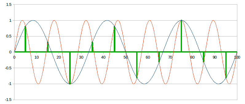
A passive attenuator is a simple voltage divider. The source device signal is a voltage swinging from + to -. Send this voltage through 2 resistors in series, R1 and R2. The downstream device receiving the signal is in parallel with R2.

The voltage will have some drop across R1, and some drop across R2. How much it drops across each resistor depends on their impedance ratios. This determines the volume setting: how much it attenuates the signal.

The passive attenuator’s volume knob has a fixed number of discrete positions, typically spaced 0.5 to 2 dB apart. For example 24 positions about 2 dB apart, or 64 positions about 0.5 dB apart. Each position puts 2 different resistors in the signal path.

Before going further, let’s mention 2 simplifying assumptions:

• The source device output impedance is zero
• The destination device input impedance is infinite

These are not actually correct, but they are close enough. Most solid state sources have output impedances around 10 to 100 ohms. Most solid state amps have input impedances around 10,000 to 50,000 ohms.

2a. Source Load

The passive attenuator shows the same load (impedance) to the source device at every volume position. So the source doesn’t “care” what volume position you are using. Make this load high enough that it is easy for the source to drive it, but no higher. The source has to swing a voltage back and forth, and the higher the load impedance, the less current it draws. So higher impedance is an easier load. But too high an impedance creates higher noise (more on that later).

A 10k attenuator means R1 + R2 = 10,000 ohms at every volume position. A 5k attenuator mean they sum to 5,000 ohms. The most popular attenuator is 10k, though 5k and 20k are also used. From here on we’ll talk about 10k, but the reasoning can be applied to any value.

As a general rule, you want at least a 1:10 ratio from the source to the load. If the source has a 100 ohm output impedance, it wants to drive a load of at least 1,000 ohms. Typical solid state sources are less than this, so a 10k attenuator gives more than 1:100 ratio which is more than sufficient. If all your sources are under 500 ohms output impedance, then you should use a 5k attenuator.

Since R1 and R2 are in series, the total load the source sees is R1 + R2. Of course it’s a little less than this since the destination device is in parallel with R2 which lowers the resistance across R2. But its input impedance is so high it doesn’t materially affect it.

So now we have the first rule of a passive attenuator: each pair of resistors R1, R2, sum to 10,000 (or 5k, or 20k).

2b. Attenuation

We mentioned earlier that the ratio of R1 to R2 determines the attenuation. Here I’ll explain exactly what that means.

At every volume position, the total load is 10,000 ohms. If R1 makes up half of that, then half the voltage drops over R1 and the other half drops over R2. In this case, if the source signal is 2 V, then 1 V drops over R1 and 1 V drops over R2. If R1 makes up 75% of that, then 75% of the voltage drops over R1 and 25% drops over R2. In this case if the source signal is 2 V, then 1.5 V drops over R1 and 0.5 V drops over R2.

We convert these ratios into dB with the standard formula

20 * log(ratio) = dB

More on that here.

It just so happens that the first example above is -6 dB of attenuation, and the second is -12 dB. That is:

20 * log(0.5) = -6
20 * log(0.25) = -12

Converting this intuition into math, this leads to the formula:

Attenuation Ratio = R2 / (R1 + R2)

Since R1 + R2 is always 10,000 this gets even simpler. If you want to attenuate the signal to, say, 17% of its original value, use a 1700 ohm resistor for R2, then R1 will be the difference between that and 10,000.

This is all there is to designing a passive attenuator — at least, to selecting the resistors for each volume position. Their ratio determines the attenuation, and their sum is always 10,000. You can get fancy and include the actual impedances for the source output and destination input, but it won’t change things much.

2c. Wrap Up

What input voltage does the downstream device see? It’s the output voltage of the attenuator. The circuit diagram makes it obvious:

The downstream device is in parallel with R2, so it sees the same voltage. The voltage drop across R2 is the output voltage, which will always be equal or less than the source voltage (since some of the voltage will drop over R1).

The diagram shows resistors for -32 dB of attenuation, or the output being 2.5% of the input.

Example: let’s compute the first few highest volume settings for a passive attenuator having 24 positions each 2 dB apart.

Position 1: full volume. Here, R1 is zero – just a straight wire and R2 is 10,000 ohms. The entire signal (2 V or whatever) drops across R2.

Position 2: -2 dB. First, compute the ratio for -2 dB. Reversing the above formula we get:

10^(-2/20) = 0.7943

This means R2 is 7,943 and R1 must be 2,057.

Position 3: -4 dB. Our ratio is 0.631, so R2 is 6,310 and R1 is 3,960.

Now resistors aren’t available in arbitrary values. You would look at the parts list and find resistors that come closest to the values you want. In practice, when designing an attenuator you can usually get the steps within 0.1 dB and keep the total resistance within 100 ohms (or 1% of your target value).

Congratulations – you can now design a passive attenuator!

The next question is: why would you use one? One part of that answer is low noise at low volume settings.

3.1 Noise

Resistors add noise to the signal. How much noise depends on the type of resistor; some are noisier than others. There is a theoretical minimum amount of noise that any resistor can have; all resistors have at least this much, in fact more. This noise has 3 common names: thermal, Johnson, and Nyquist. But whatever you call it, it is the same thing: the heat energy from the resistor’s temperature, randomly exciting electrons that appear as tiny voltages. We’re talking super tiny here. For our application, it is in micro-Volts (millionths of volts). This noise spans all frequencies, so the amount of noise that is relevant to our application depends on the bandwidth. In audio, let’s assume bandwidth is 20,000 Hz.

A passive attenuator introduces other kinds of noise too. Resistor composition noise, junction/contact noise, etc. To minimize these noises, use high quality contacts and “clean” resistors. The cleanest resistors are wire wound and metal film. These resistors have actual real-world noise so close to the theoretical minimums, we can use those minimums in our noise computations. This isn’t true of other resistor types, which are noisier.

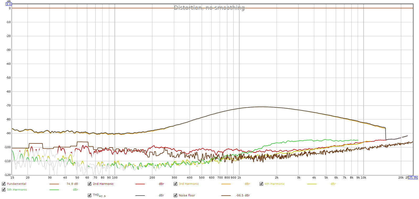
For example, thermal noise of a 10,000 ohm resistor at room temperature in audio bandwidth is about 1.8 uV, or 1.8e-6 volts. A 100 ohm resistor is 0.18 uV, or 1.8e-7 volts. Dropping the resistance by a factor of 100 drops the noise by a factor of 10. If the signal (voltage drop) over the resistor is 1 V, this is -115 and -135 dB SNR respectively. The first is comparable to the noise in the very best active preamps, the second is better than any active preamp. However, if we reach a quiet part of the music and the signal drops 30 dB quieter, the noise level remains constant so the SNR drops by 30 dB and it’s 85 dB and 105 dB respectively.

3.1.1 Noise: Absolute or Relative

When you use a thermal noise calculator you’ll find that resistor noise is measured in 2 ways: as a voltage, and as a voltage ratio. The astute reader will wonder: It can’t be both, so which is it? In other words: Is resistor noise inherently a ratio, so if you apply a smaller voltage across the resistor you get less noise, and the SNR remains constant? Or is resistor noise inherently a constant, so if you apply a smaller voltage across the resistor, the signal is smaller relative to the noise and the SNR drops?

Sadly, for our purposes building passive attenuators, resistor noise is inherently a constant. It is the same regardless of the voltage across or current through the resistor. This suggests that noise is unlikely to be an issue at max volume, but it may become an issue as we turn down the volume.

3.1.2: Noise From What Resistor?

OK so we can compute noise but we’re still not out of the woods. When computing the noise added by a passive attenuator, it’s not obvious which resistor, or more generally what impedance, to use!

For example consider the above circuit diagram. The signal passes through both R1 and R2, so intuition says each one adds noise and the total noise should be the sum of the noise from each. But that sum is always 10,000 ohms, so the noise would always be 1.8e-6 volts. But this simple intuitive approach is incorrect.

3.1.3: Output Impedance

The solution is to view this from the perspective of the destination device. Just like the voltage that matters is the voltage across the destination device’s terminals, the impedance that matters for noise computation is the impedance that the destination device sees. This is called the output impedance of the passive attenuator. Imagine you are at the input terminals of the destination device looking upstream toward the source. What impedance do you see?

Going from + to – upstream, you see R2 in parallel with (R1 and source output impedance in series) . In other worse, the passive attenuator’s output impedance is:

1 / ((1 / R2) + ((1 / R1 + SourceOutput)))

Since output impedance is typically very small, this is close to R2 and R1 in parallel, which is:

1 / ((1 / R1) + (1 / R2))

When R2 and R1 are very different, this is roughly equal to the smaller of them. When R1 and R2 are nearly equal, this is roughly equal to half of either of them.

This is the impedance that determines the noise added by the passive attenuator.

Important note: remember the requirement that the destination device have a high input impedance? You want another 1:10 ratio here. That is, the input impedance of the amp (or your downstream destination device) should be at least 10 times higher than the output impedance of the passive attenuator. The worst-case highest output impedance is when R1 and R2 are equal, 5,000 ohms each at -6 dB. Here the output impedance is 2,500 ohms. So the amp should have an input impedance of at least 25 kOhm.

If it doesn’t, then use a 5k attenuator. But the lower impedance makes it harder to keep the 1:10 ratio on the input side. However, it’s still pretty generous since most solid state sources have output impedances well under 500 ohms.

3.1.4 Computing Noise

Let’s compute the passive attenuator noise from our example above at 0 dB, -2 dB and -4 dB.

At 0 dB, the 2 output impedance legs are 10,000 ohms, and zero. Well not quite zero, but the output impedance of the source device. Let’s suppose that’s 100 ohms. The output impedance will be close to 100 ohms. But more precisely:

1 / ((1 / 10000) + (1 / (0 + 100))) = 99 ohms

Thermal noise of 99 ohms (at room temp and audio bandwidth) we’ve already computed above at 1.8e-7 volts. Also at 0 dB we have the full scale signal from the source, which is 2 V at its loudest which gives us a SNR of:

20 * log(1.8e-7 / 2.0) = -141 dB

Wow! No active preamp achieves that! And it’s probably even better because the output impedance of solid state sources is usually closer to 1 ohm than 100 ohms.

Let’s check the SNR when the music (source voltage level) reaches a quiet part, say 30 dB lower, which is 63.2 mV. Note: we’re not turning down the attenuator, it’s still at 0 dB. We’re just passing a quieter musical signal through it.

20 * log(1.8e-7 / 0.0632) = -111 dB

Well, we really didn’t have to do the math there. Thermal noise is constant and the signal dropped by 30 dB, so the SNR drops by 30 dB. That’s a big drop, but it’s still very good. Again, it’s probably better in the real world because it depends on the the source output impedance will will probably be closer to 1 ohm than 100.

At -2 dB the R1 & R2 resistors are 2,057 and 7,943 ohms. The output impedance will be:

1 / ((1 / 7,943) + (1 / (2,057 + 100))) = 1,696 ohms

Thermal noise of 1,696 ohms is 7.41e-7 V. Per the above, at -2 dB the output is 79.43% of the input. So voltage across R2 (the output voltage) for a 2 V source signal is 1.5886 V. Thus the SNR is:

20 * log(7.41e-7 / 1.5886) = -127 dB

If the music reaches a -30 quiet part, it’s 30 dB worse which is -97 dB.

Now let’s skip -4 dB and use a more realistic listening level. Nobody listens that loud. Typical attenuation for actual listening with a power amp or headphones is around -30 dB. Of course this is a very rough figure depending on amp gain, speaker efficiency, room size and listener preferences. But it’s in the ballpark.

At -30 dB the attenuation is:

10 ^ (-30/20) = 0.03162

So the R2 resistor must be 3.162% of 10,000 which is 316 ohms. That means R1 must be 9,684 ohms. This means the output impedance is:

1 / ((1 / 316) + (1 / (9,684 + 100))) = 306 ohms

Thermal noise at 306 ohms is 3.15e-7 V. At -30 dB the output is 3.162% of the input. So voltage across R2 for a 2 V source is 0.06324 V. Thus the SNR is:

20 * log(3.15e-7 / 0.06324) = -106 dB

And if the music reaches a part 30 dB quieter, that’s -106 – 30 = -76 dB.

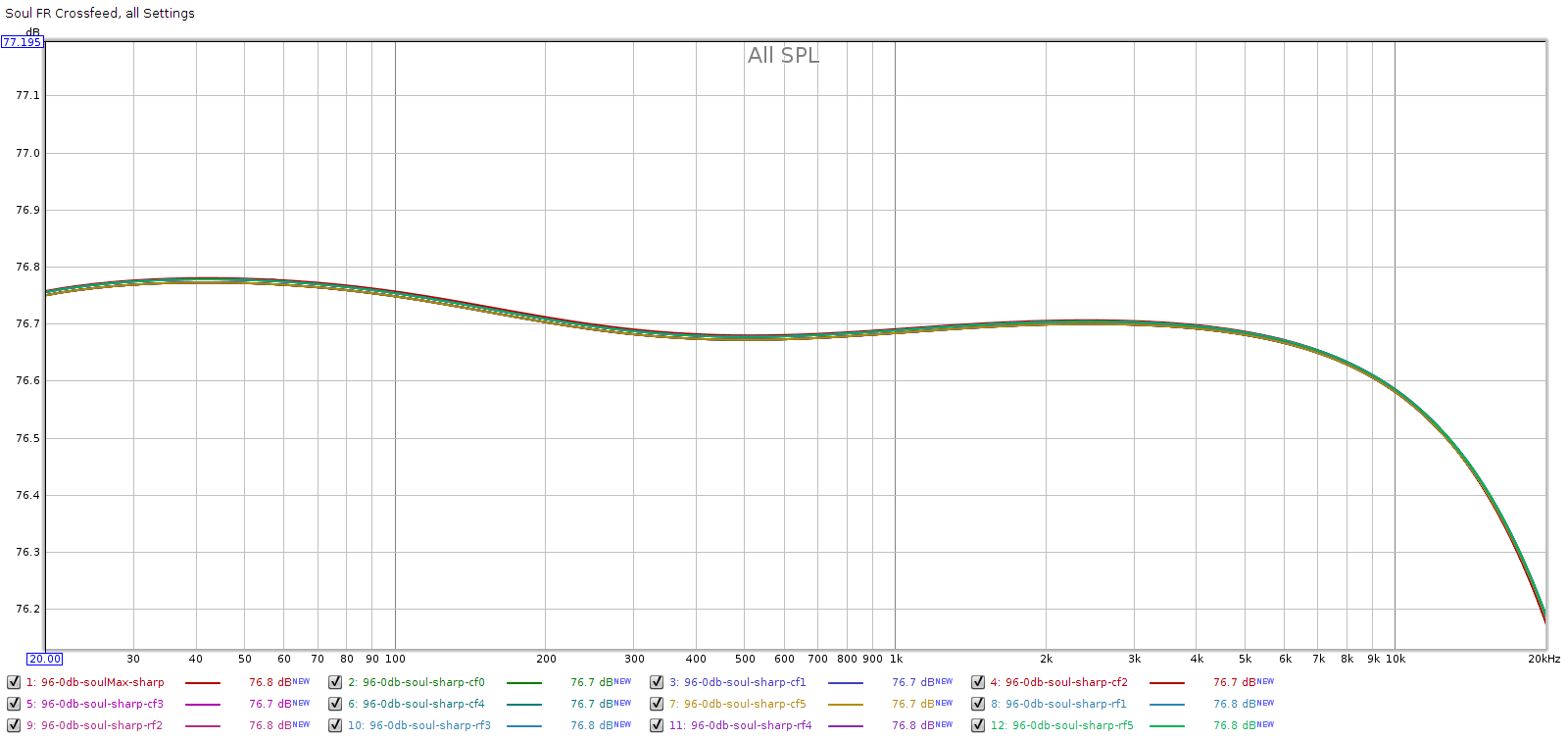
3.2 Frequency Response

Some people say passive attenuators have perfectly flat frequency response. Indeed, why wouldn’t they? They’re simple voltage dividers made of metal film resistors, and resistors have perfectly flat frequency frequency response! Alas, it’s not that simple.

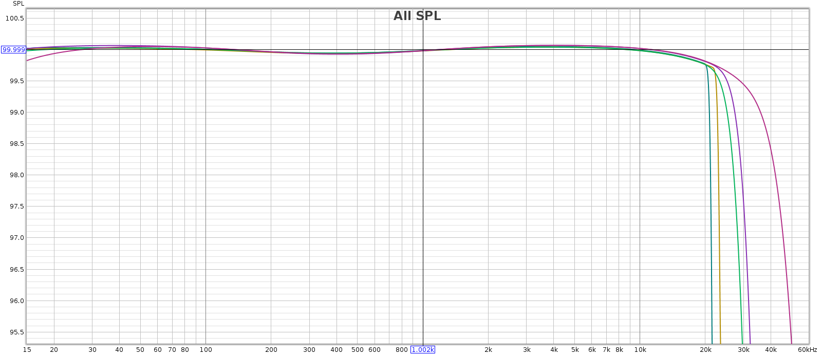
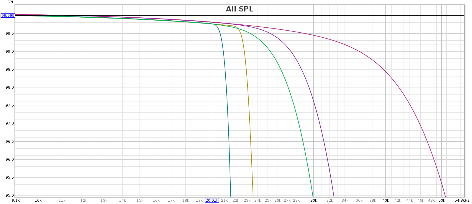
A passive attenuator is connected to a downstream device. The cables that connect it have some capacitance, and the attenuator’s output impedance combines with this capacitance to form an R-C circuit that acts as a low-pass filter. Put differently, the capacitance carries high frequencies to ground before they reach the downstream device. So the key question: what is the bandwidth of this filter?

Bandwidth is typically defined by the -3 dB point, which is the lowest frequency at which it attenuates by 3 dB. This has a simple equation:

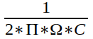
That is, it’s inversely proportional to the product of output impedance and cable capacitance. Because this defines the upper frequency response of the attenuator, we want this to be as big as possible. That means we want both output impedance and capacitance to be a small as possible.

So let’s plug in typical numbers. As explained above, the worst-case output impedance of our 10k attenuator is 2500 ohms (1250 ohms for a 5k attenuator). For cable, let’s take Blue Jeans LC-1, which is high quality yet inexpensive. Its capacitance is 12.2 pF per foot. That’s 12.2 pico-Farads, or trillions of a Farad = 12.2 * 10^-12 Farads. With 6 feet of this cable between the passive preamp and downstream device, we have 12.2 * 6 = 73.2 pF of capacitance.

The above formula gives us 870,000, or 870 kHz. That’s the frequency at which this passive attenuator is down 3 dB. And that is the worst-case! For example at -30 dB attenuation, the output impedance is 306 ohms so the bandwidth is 7.1 MHz.

In short, the passive attenuator has perfectly flat frequency response in the audible spectrum. It’s true that a passive attenuator can attenuate frequencies in the audible spectrum, but this concern is more theoretical than practical. That would take ridiculously high capacitance (poorly engineered) cables or long runs. In our example, to bring the -3 dB point down to 20 kHz you can compute it would require about 260 feet of cable!

4. Comparison to Active Preamps

Most active preamps have a fixed gain stage with attenuation. Usually the attenuation is upstream from the gain, because that helps prevent input voltage clipping. But it has the drawback that any noise added by the attenuation potentiometer is amplified by the gain ratio. Furthermore, the amount of noise, which depends largely on the gain ratio, is constant regardless of the signal level. This means as you turn down the volume, the SNR drops with it.

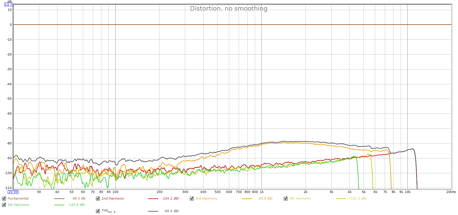
The SNR of amps and preamps is measured at full output. But this is misleading, since nobody actually listens at full output. When was the last time you listened to music with the volume set to full blast? With typical listening levels 20 to 40 dB below full output, the SNR you actually hear when listening is 20 to 40 dB less than advertised.

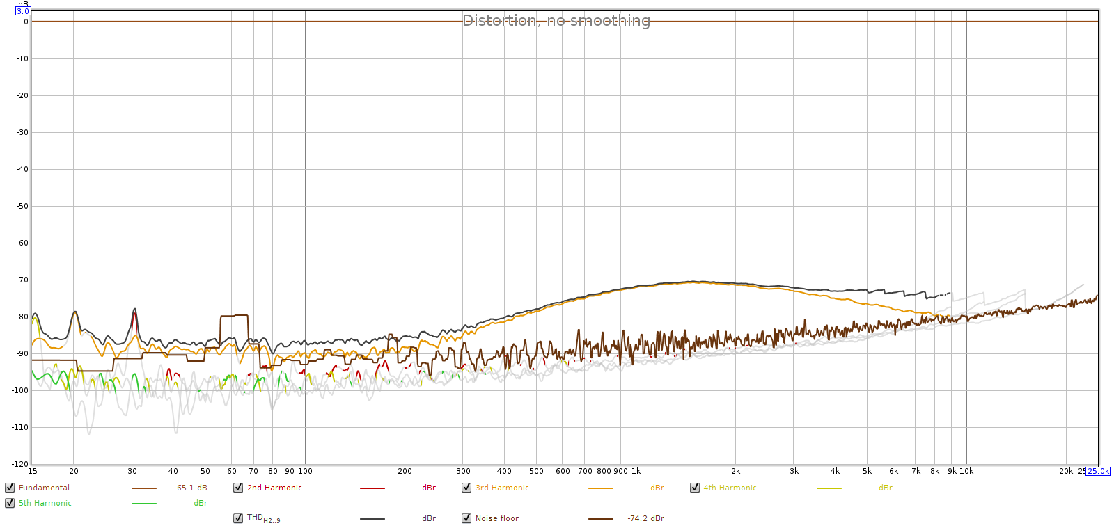
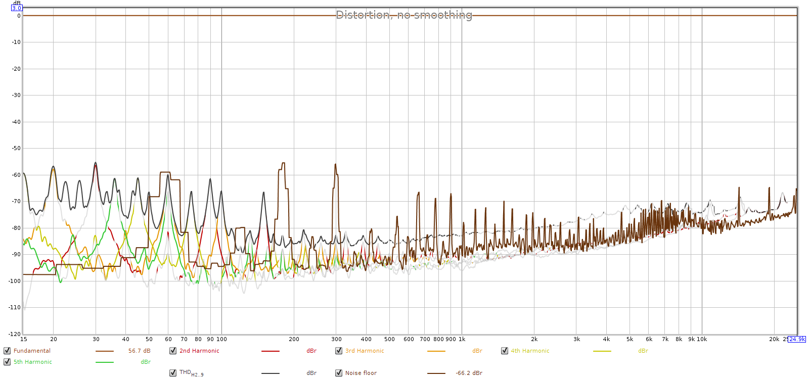
You can see this in practice on many of the reviews at Audio Science Review. The SNR at 50 mV output is typically 30-40 dB lower than the SNR at full volume. With full volume normally being 2 V, that’s 32 dB of attenuation giving 30-40 dB worse SNR.

Consider an ultra-high quality active preamp having an SNR of 120 dB at full scale 2.0 V output. When you turn it down to a typical listening level, say -30 dB, the SNR drops to the mid 80s. If you took the full scale output of that preamp and sent it to a passive attenuator having the same 30 dB of attenuation, the SNR would be 106 dB. The passive attenuator is 20 dB quieter than the active preamp.

In summary, at full volume a passive attenuator has no advantage. But at the lower levels that we actually listen, they have:

• Lower noise.
• Lower distortion.
• Perfectly flat frequency response at audio frequencies.

Of course, this assumes the system meets the requirements listed earlier (most systems do).

4.1 Exceptions

Here are the exceptions that prove the rule. Some active preamps are designed for improved performance (lower noise) at low volume settings.

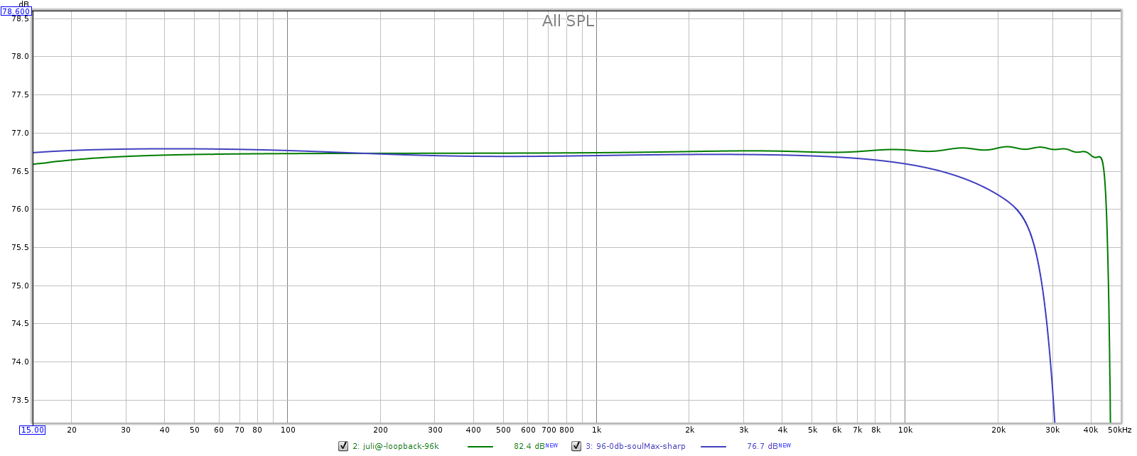
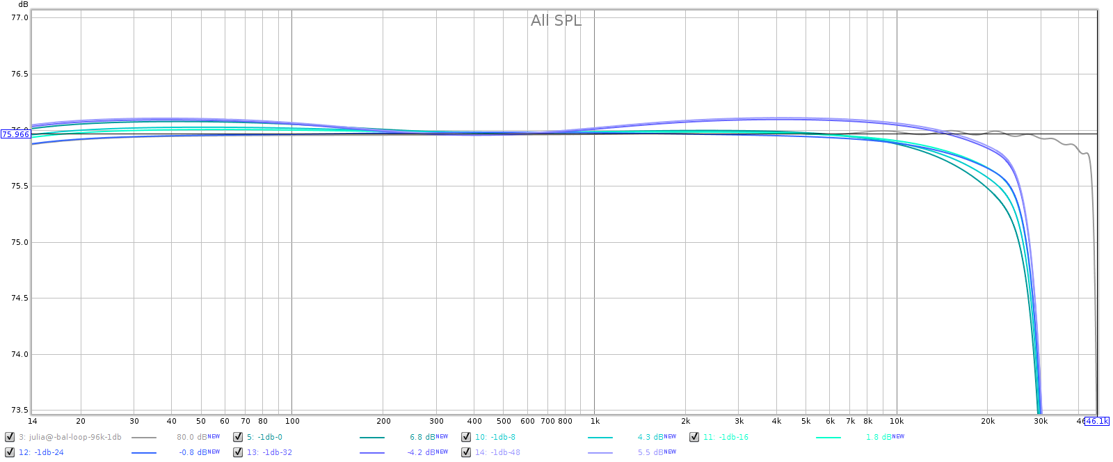
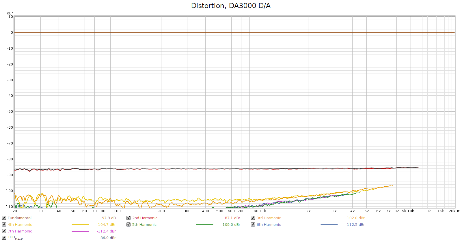
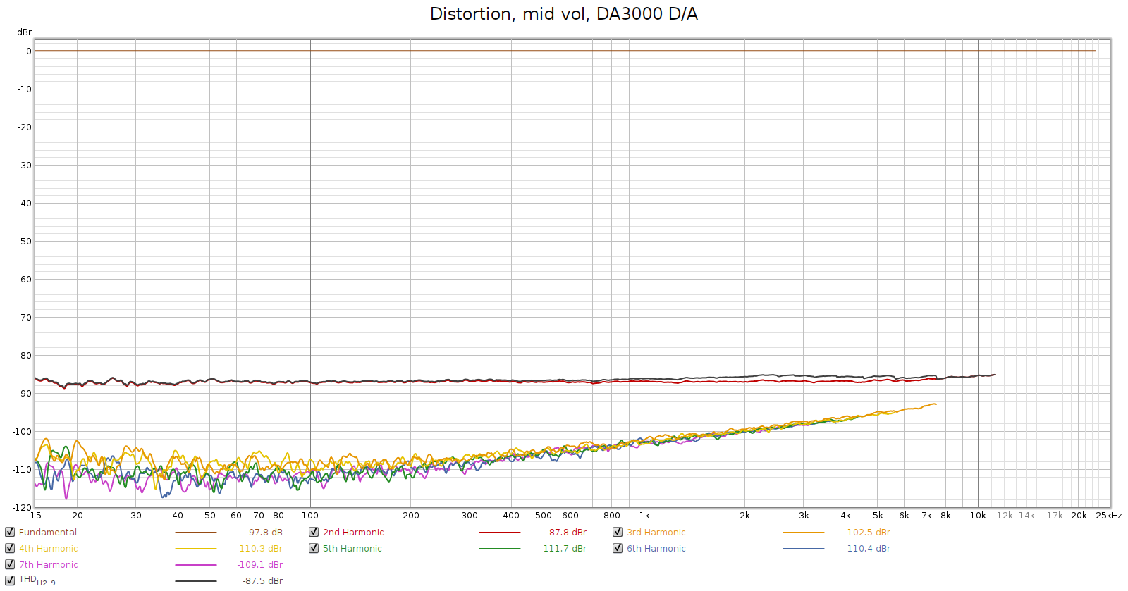
One way is to put the volume potentiometer downstream from the gain stage. This has 2 advantages: first, pot noise is not amplified by the gain ratio. Second, it attenuates the signal after the gain noise has been added, so it attenuates both the signal and the noise. The drawback is that this exposes the gain stage directly to the source voltages, so it will clip if those voltages are too high. The JDS Atom is an example of this design and it has great low volume performance. At 2 V its SNR is 120 dB, and at 50 mV it is 92 dB. As you turn the volume down by -32 dB, the SNR drops by 28 dB. This is less than 1:1, where most preamps are more than 1:1.

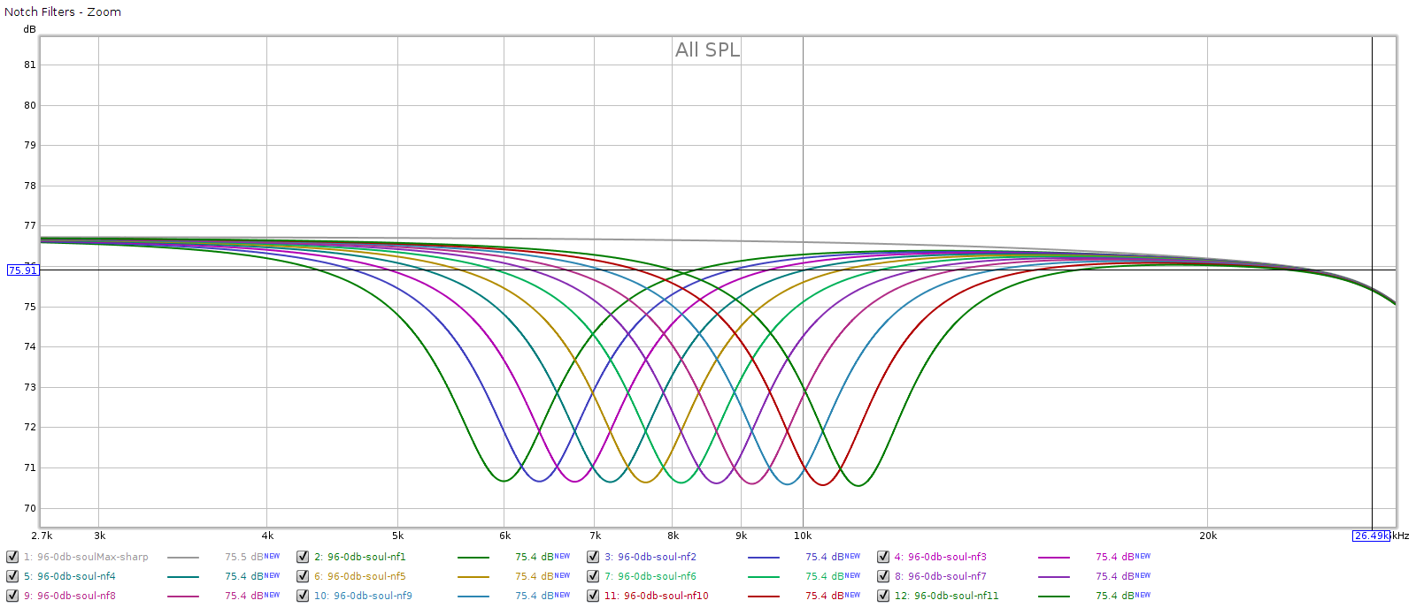
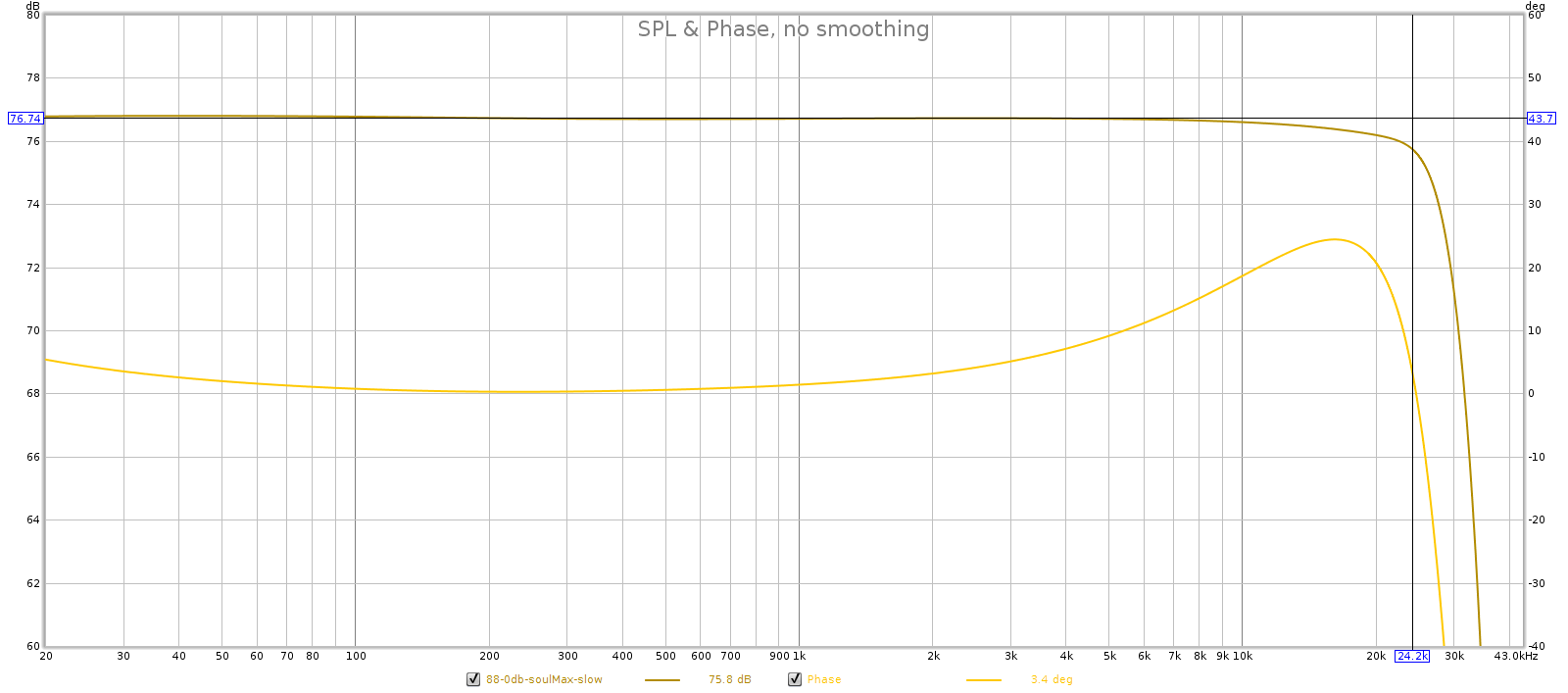
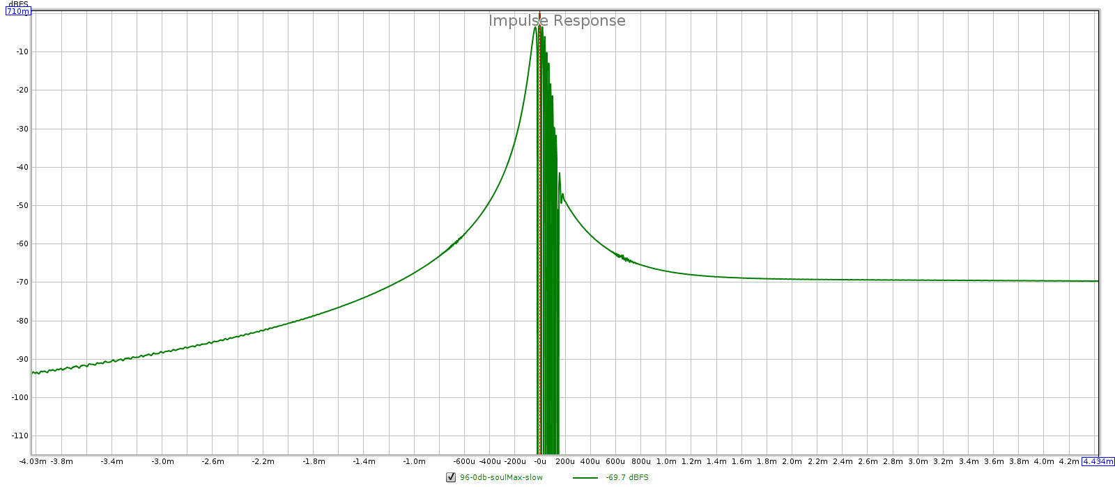
Another way is for the preamp to change its gain ratio, instead of using a fixed gain ratio with attenuation. As you turn down the volume, you reduce the gain ratio, which reduces noise & distortion (and widens bandwidth). This requires less than unity gain, which can be done with an inverting gain-feedback loop. Of course, this entirely obviates the need for separate attenuation. The volume control changes the “R1” and “R2” metal film resistors in the gain-feedback loop. This is an unusual design that some Meier Audio amps use, and they have the lowest noise I’ve measured — the Corda Soul measures even lower noise than the JDS Atom.

In summary, at the low to medium volumes we actually use for listening, a passive attenuator has better SNR than conventional active designs. But there are a few actives of unusual design that can equal or exceed the performance of a passive.

Background

Most of the sounds we hear are made up of many different frequencies all vibrating together at the same time. The energy in a wave depends on its amplitude and frequency. The higher the amplitude, the more energy. Also the higher the frequency, the more energy. The amplitude part of this makes intuitive sense. The frequency part does too, but it is less obvious.

If the energy of a wave depends on its amplitude and frequency, this implies that if total energy is constant for all frequencies, then amplitude must drop with frequency.

Consider a musical instrument playing a sound. Since energy depends on amplitude and frequency, if it puts equal energy into all the frequencies it emits, then the higher frequencies must have a smaller amplitude. Musical instruments don’t actually put equal energy at all the frequencies they emit, but this does hold true roughly or approximately. If you do a spectrum analysis, they are loudest at or near the fundamental (lowest) frequency and their amplitude drops with frequency. Typically, roughly around 6 dB per octave. That is, every doubling of the frequency roughly halves the amplitude.

For example, here is amplitude vs. frequency for a high quality orchestral recording:

This graph shows amplitude dropping as frequency increases. Since energy is based on amplitude and frequency, this means roughly constant energy across the spectrum (all frequencies).

This implies that low frequencies are responsible for most of the amplitude in a musical waveform. So, if you look at a typical musical waveform, it looks like a big slow bass wave with ripples on it. Those ripples are the higher frequencies which have smaller amplitudes. Further below I have an example picture.

Audio Linearity

Audio devices are not perfectly linear. They are usually designed to have the best linearity for medium level signals, and as the signal amplitude approaches the maximum extremes they can become less linear. This is generally true with analog devices like speakers and amplifiers, and to a lesser extent with digital devices like DACs.

For example, consider a test signal like 19 and 20 kHz played simultaneously. If you encode this signal at a high level just below clipping, it’s not uncommon for DACs to produce more distortion than they do for the same signal encoded just a little quieter. I’ve seen much smaller level changes, like a 1 dB reduction in level giving a 24 dB reduction in distortion! The same can be true for amplifiers.

Incidentally, when companies publish specs for DACs or CD players, they typically measure distortion at around -20 dB. Yet they measure noise or SNR at full scale. So they’re not really telling the whole truth.

Furthermore, the lower the level of a sound, the fewer bits remain to encode it. 16-bit audio refers to a full scale signal. But a signal at -36 dB has only 10 bits to encode it because the 6 most significant bits are all zero. Because in music the high frequencies are at lower levels, they are encoded with even fewer bits, which is lower resolution. In our -36 dB example, high frequencies 3 octaves above the fundamental are likely 18 dB smaller, which is only 7 bits. When we consider that the lowest bit is dither, this is only 6 bits for the frequencies where our hearing is most sensitive!

The Redbook CD standard had a solution to this called pre-emphasis: boost the high frequencies before digital encoding, then cut them after decoding. This was an effective solution but is no longer used because it reduces high frequency headroom and most recordings today are made in 24 bit and are dithered when converted to 16-bit.

The Importance of Bass Response

One insight from the above is that bass response is more important than we might realize. At low frequencies (say 40 Hz), the lowest level of distortion that trained listeners can detect is around 5%. But at high frequencies (say, 2 kHz), that threshold can be as low as 0.5%.

So one could say who cares if an audio device isn’t perfectly linear? Because of the energy spectrum of music, the highest amplitudes that approach non-linearity are usually in the bass, and we’re 10 times less sensitive to distortion in the bass, so we won’t hear it.

But this view is incorrect. It is based on faulty intuition. The musical signal is a not a bunch of frequencies propagating independently. It is a single wave with all those frequencies superimposed together. Thus, the high frequencies are riding as a ripple on the bass wave. If the bass wave has high amplitude approaching the non-linear regions of a device, it is carrying the smaller amplitude high frequencies along with it, forcing even those smaller frequencies into the non-linear region.

A picture’s worth 1,000 words so here’s what I’m talking about, a snippet from a musical waveform. The ripples marked in red are the midrange & treble which is lower amplitude and normally would be centered around zero, but riding on top of the bass wave has forced them toward the extreme positive and negative ranges:

Speaker Example

Here’s another practical example. Decades ago, I owned a pair of Polk Audio 10B speakers. They had two 6.5″ midrange drivers, a 1″ dome tweeter, and a 10″ tuned passive radiator. The midrange drivers produced the bass and midrange. As you turned up the volume playing music having significant bass, at some point you started hearing distortion in the midrange. This is the point where the bass energy is driving the 6.5″ driver excursion near its limits where its response goes non-linear. All the frequencies it produces are more or less equally affected by this distortion, but our hearing is more sensitive in the higher frequencies so that’s where we hear it first.

Obviously, if you turn down the volume, the distortion goes away. However, if you use EQ or a tone control to turn down the bass, the same thing happens – the distortion goes away. Here the midrange frequencies are just as loud as before, but they’re perfectly clear because the distortion was caused by the larger amplitude bass wave forcing the driver to non-linear excursion.

Other Applications: Headphones

The best quality dynamic headphones have < 1 % distortion through the midrange and treble, but distortion increases at low frequencies, typically reaching 5% or more by the time it reaches down to 20 Hz. The best planar magnetic headphones have < 1% distortion through the entire audible range, even down to 20 Hz and lower. This is due in part to having a physically large driver, which moves less to produce a given volume level.

Most people think it doesn’t matter that dynamic headphones have higher bass distortion, because we can’t easily hear distortion in the bass. But remember that the mids and treble are just a ripple riding on the bass wave, and most headphones have a single full-range driver. If you listen at low levels, it doesn’t matter. But as you turn up the volume, the bass distortion will leak into the mids and treble and become audible.

Thus, low bass distortion is more important in a speaker or headphone, than it might at first seem. If the headphone or speaker has a separate bass driver with a crossover, then this doesn’t apply – the mids and treble aren’t affected by the bass excursions.

Test signals like frequency sweeps will not show this increased distortion, because they don’t play bass & treble at the same time.

Other Applications: amplifiers and DACs

Amplifiers and DACs have a similar issue, though to a lesser extent. This concept applies here as well – especially when considering the dynamic range compression that is so often applied to music these days.

Consider a digital recording that is made with dynamic range compression and leveled too hot, so it has inter-sample overs or clipping. Or, it may be perfectly clean, but with levels that are just below full scale. Sadly, this describes most modern music rock/pop recordings, though it’s less common in jazz and classical.

Most of the energy in the musical waveform is in the bass, so if you attenuate the bass you reduce the overall levels by almost the same amount. This will entirely fix inter-sample overs, though it can’t fix clipping. Remember the 19+20 kHz example above, showing that distortion increases as amplitude levels approach full scale? With most music, attenuating the bass will fix that too, since the higher frequencies are usually riding on that bass wave. For example, this explains how the subsonic filter on an LP may improve midrange and treble response.

The Corda Soul uses the WM8741 DAC chip. Actually, it uses 2 of them, each in mono mode which gives slightly better performance. This chip has 5 different anti-aliasing reconstruction filters. The Corda Soul has a switch to select either of 2 different filters. Here I describe these filters, show some measurements I made, and from this make an educated guess which 2 of these filters the Corda Soul uses, at various sampling rates. At higher sampling frequencies the digital filter should make less difference; more on that here. My measurements and observations below are consistent with that.

Note: this DAC chip has a mode called OSR for oversampling. The Soul uses this chip in OSR high, which means it always oversamples the digital signal at the highest rate possible, to 192 or 176.4 kHz, whichever is an integer multiple of the source. For example, 44.1k is oversampled 4x to 176.4k and 96k is oversampled 2x to 192k. The function of the digital filters depends on this OSR mode.

Summary: the filters have 3 key attributes:

• Frequency Response: how fast (sharp) or slow they attenuate high frequencies.
• Frequency Response: the filter stop-band – is it above, at, or below Nyquist.
• Phase: whether the filter is linear (constant group delay, FIR) or minimum phase (variable group delay, IIR).

This table summarizes key filter attributes – taken from the WM8741 data sheet linked above, for 44.1k / 48k sampling in OSR high mode.

Note: at 44.1 kHz sampling, filters 1 and 3 are almost identical. The first is called “soft knee” while the third is called “brickwall”. Yet strangely, their frequency response is the same (despite their names which suggest otherwise) and the only difference is that 1 has more group delay. This suggests that the labels for filters 1 and 2 might have been mistakenly reversed in the WM8741 data sheet. Brickwall is usually the standard sharp filter closest to the ideal mathematical response. But not here, because being only -6 dB at Nyquist, it can allow ultrasonic noise to leak into the passband.

Filters 4 and 5 are labeled as apodizing. From what I read, this means their stop-band is a little below Nyquist. Why set the stop-band below Nyquist? Theoretically this is unnecessary. The reason given is that rejecting the upper band just below Nyquist is supposed to be an extra-safe way of avoiding any distortion introduced by the AD conversion during recording. Here, the stop-band of the apodizing filters is at Nyquist, but that’s still a bit lower than the others which are above Nyquist (which is an improper implementation).

Based on the above chart, filter 5 is the most correct implementation because it is the only filter that is fully attenuated by Nyquist, with flat phase response (minimal group delay). However, filter 5 rolls off a little early to achieve this. If you want flat response to 20 kHz, filter 3 is the best choice, though it does so at the price of allowing some noise above Nyquist. If one wanted a minimum phase alternative, the best choice would be filter 4. Both 1 and 4 are minimum phase, but 1 is not fully attenuated at Nyquist. Filter 4 is. However, to achieve this, filter 4 sacrifices FR with an earlier roll off.

For comparison, here’s how these filters behave at 96k / 88.2 k sampling (also in OSR high mode).

At these higher sampling rates, all the filters are fully attenuated by Nyquist (or lower). That’s a good thing and Wolfson should have done this at the lower rates too. Also, filters 1, 2, 4 and 5 (all but 3) take advantage of the higher sampling frequency to have a wide transition band with gentler slope. This sacrifices response above 20k (which we don’t need) to minimize passband distortion, particularly phase shift. The numbers reflect this, as they all have flatter (better) phase response than filter 3.

As with the first table, filters 1 and 2 look like a mis-print; both have the same transition and stop bands. But all else equal, linear phase should have less phase shift, not more. This is probably a typo, because as you’ll see below, the impulse response for filter 1 is asymmetric, and for filter 2 is symmetric, and symmetric impulse response usually implies linear phase.

Based on this data, filters 2, 3 or 5 are the most correct implementations. Filter 3 has flat FR up to 40 kHz, but this extra octave comes at the price of a narrower transition band having more phase shift and group delay. Filters 2 and 5 have flatter phase response but start rolling off around 20 kHz to get a wider transition band. If one wanted a minimum phase alternative, filters 1 or 4 are the only choices and either would be fine.

I measured the Soul’s output with the digital filter switch in each mode, sharp and slow, using 2 test signals: a frequency sweep and a square wave. From this, I measured frequency and phase response, group delay and impulse response. Charts/graphs are below, in the appendix.

Here’s the square wave: first sharp, then slow:

Overall, at 44.1 kHz I observed 3 key differences:

1. In sharp mode, frequency response and group delay are both flat to 20 kHz.
2. In slow mode, frequency response starts to roll off and group delay starts to rise between 18 and 19 kHz.
3. In slow mode, the square wave shows no ripple before a transition, and ripples with greater amplitude and longer duration after a transition.
4. The above curves are similar when comparing the sharp & slow filters at 48k sampling.

From these observations I conclude that for 44.1k and 48k signals, the Soul uses filters 3 and 4 in sharp and slow modes, respectively. Here’s why:

• Because FR is flat to 20 kHz in sharp mode, it must be using filter 1 or 3.
• Because GD is flat in sharp mode, it must be using filter 3.
• Because FR rolls off just above 18k in slow mode, it must be using filter 2, 4 or 5.
• Because GD rises in slow mode, it must be using filter 4.

Appendix

I recorded these graphs using my sound card, an ESI Juli@. This is not a great setup, but it’s the best I can do without dedicated equipment.

PC USB Audio output –> Corda Soul USB input –> Corda Soul analog output –> sound card analog input

Details:

• Configured the sound card for analog balanced input & output (flip its daughter board from unbalanced to balanced.
• Cabled from Soul to Juli@, using 3-pin XLR to 1/4″ TRS.
• On PC:
  • Disable pulseaudio
  • Use Room EQ Wizard (REQW) on PC, in ALSA mode
  • Configure REQW
    • set desired sampling rate (44.1, 48, 88.1, 96)
    • set audio output to USB
    • set audio input to Juli@ analog
  • Configure Corda Soul
    • Select USB audio input
    • Ensure all DSP disabled (knobs at 12:00)
    • Set volume as desired
      • measured at max: 0 dB
      • measured at 12:00; -16 dB; 34 clicks down
  • Use REQW “Measure” function
  • Confirm proper sampling rate light on Corda Soul

Important Note: My measurements depend as much on the Corda Soul as they do on the Juli@ sound card. For example, if the Juli@ rolls off the frequency response faster than the Soul, then I will measure the same FR in both mods of the Soul. And if the Juli@ applies a minimum phase filter that adds phase distortion, then I will measure that phase distortion in both modes of the Soul. This probably explains why the digital filter responses were so similar at 88 and 96 kHz.

Here are FR, phase, GD and impulse plots for all tested sampling rates. Each is sharp top, slow bottom. Observe that at multiples of 44.1k (44.1k and 88.2k), the sharp filter has flat phase response while the slow filter does not. But at multiples of 48k (48k and 96k), both filters have similar non-flat phase response. This is probably due to the Juli@ card. However, the comments below assume the Juli@ card is transparent and all differences are due to the Soul.

In all cases, both filters at all sampling rates:

• Frequency response: starts to taper at 20 kHz for the widest possible transition band.
• Impulse response: sharp is symmetric, slow is asymmetric.
• Group delay: sharp is flatter than slow.
• At high sampling rates, the difference between the filters becomes immaterial. This is consistent with theory.

44.1 kHz: sharp is filter 3 and slow is filter 4.

• Sharp FR doesn’t taper until past 20k, so it must be filter 1 or 3.
• Sharp has flat GD, so it must be filter 3.
• Slow FR tapers past 19k, so it must be filter 4 or 5.
• Slow has more GD than sharp, so it must be filter 4.

48 kHz: sharp is filter 3 and slow is filter 4, for the same reasons as above.

88.2 kHz: Sharp is filter 2 and slow is filter 1.

• Both FR start to taper at 20 kHz, so neither can be filter 3.
• Both have a stopband at 44,100 kHz (beyond 40k), so neither can be filter 4 or 5.
• Sharp has flatter phase / less group delay, which is filter 2.

96 kHz: Sharp is filter 2 and slow is filter 1.

• Both FR start to taper at 20 kHz, so neither can be filter 3.
• Both have a stopband at 48 kHz (beyond 44k), so neither can be filter 4 or 5.
• Sharp has flatter phase / less group delay, which is filter 2.

I own this headphone amp and use it every day at work. It has great sound quality with some unique features. I previously reviewed it and compared with other amps here.

Earlier this year I loaned this amp to Amir to measure for Audio Science Review, here. Amir does a great service to the audiophile community, I’ve met him in person and he’s a good guy with industry experience and a knowledgeable audiophile. However, we are all human with different opinions, and even objective measurements can be misleading.

Take SNR (signal:noise ratio) and SINAD (Signal over Noise and Distortion) for example. These are typically measured at a device’s full scale output, as this usually gives the highest number. But with headphone amps, we don’t listen at full volume. Their max output level is around 2-4 Vrms, sometimes more. This is far too loud for average listening levels; it would be painful or cause hearing damage. We typically listen with average levels around 70 or 80 dB SPL, which, perceptually, most people would describe as medium-loud. Most headphones reach this level with a voltage around 50 mV.

For example, consider the Matrix Audio Element, which Amir recently reviewed. It is one of the best DACs he’s ever measured, with a SINAD of 120 dB. However, its 50 mV SINAD is only 81 dB.

For comparison, The Corda Jazz measured about 87 dB SINAD at full output, and 90 dB at 50 mV output.

This illustrates an important point. We start with 2 devices. One has a SINAD of only 87 dB, which seems low. The other has a SINAD of 120 dB, which is the best he’s ever measured. Objective measurements tell us one is better! However, that is highly misleading because when you measure the output at levels we actually use, the exact opposite happens. The Jazz is actually 9 dB better than the Matrix. That’s a 65% drop in noise & distortion, which is a significant, audible improvement.

In short, the max SINAD measurement is correct, but misleading because it describes conditions that nobody actually uses when listening. The 50 mV SINAD is a better measurement because it represents actual listening conditions. But virtually nobody measures this; Amir (much to his credit) is the only person I know of who does this. Furthermore, the large variance between these two belies their similarity: as in the above example, the devices measuring the highest peak SINAD often do not measure the highest 50 mV SINAD, which proves how important it is to understand the measurements we make and their relevance to what we hear.

Enough said about this. Next I’ll talk about how the way an amp is designed affects this. If you don’t care about engineering details just skip to the conclusion.

Lesson learned: an amplifier’s SNR or SINAD can be quite different at 50 mV than it is at full output. How does this happen? The conventional amplifier has its internal gain-feedback loop set to whatever fixed gain ratio produces the desired maximum output, and the volume control is a potentiometer (variable resistor) that attenuates this. This “fixed gain with attenuation” means the noise level is relatively constant (based on the gain ratio, which is fixed), so as you turn the volume down, you reduce the SNR and SINAD at the same time.

This is easily seen with the Matrix. Full output is 3.9 V, so 50 mV is 38 dB quieter. And its 81 dB 50 mV SINAD is 39 dB less than 120 dB. What a coincidence: turn the volume down by 38 dB and SINAD drops by 39 dB! They have a virtually perfect 1:1 relationship. Not a coincidence; that’s by design.

So what’s happening with the Jazz? Its SINAD actually gets better at lower volumes. The Jazz is designed differently from typical amps. It does not use fixed gain with separate attenuation, but instead it uses variable gain to set the attenuation you need, obviating any need for separate attenuation.

The Jazz volume control changes the resistors in its internal gain-feedback loop. At low volumes, it has less gain and more negative feedback (wider bandwidth, lower noise and distortion). As you turn up the volume, you are increasing the gain (reducing negative feedback). [Incidentally, this means it must be inverting, for its gain-feedback loop to have less than unity gain. But its final fixed-gain stage is also inverting, so overall it does not invert.] Finally, this volume control is not a potentiometer; there is no potentiometer in the signal path.

This means the Jazz produces its best sound quality at the low to medium levels we actually use for listening. It also means the Jazz has perfect channel balance at every volume setting. Another observation from Amir’s measurements is that the Jazz is not current limited. It puts out 10x more power into 30 ohms, than 300 ohms.

Conclusion

Amir didn’t like the Jazz in his review, mainly because of its limited output power. One of the limitations of the Jazz’s unique volume control is that the resistors in the gain-feedback loop can only handle limited voltages. If you turn up the volume too high, it produces huge amounts of audible distortion due to input stage voltage clipping. The Jazz maximum output level before the onset of this clipping & distortion is about 3.7 V. That equates to 116 dB SPL with Sennheiser HD-580 and 120 dB on Audeze LCD-2. This is more than loud enough for me. Anyone listening this loud risks damaging his hearing. In fact, with the LCD-2 headphones I use the Jazz in low gain mode which is 16 dB quieter than this.

In summary, the Jazz is an amp that Amir’s measurements show has perfectly flat frequency response, perfect channel balance at all volume settings, less than 1 ohm output impedance (not current limited), and SINAD among the best he’s ever measured, at actual listening levels (50 mV). Yet he doesn’t recommend this amp because of its limited output voltage. At the same time, he does recommend amps like the Matrix, which have higher output power, but inferior measurements at the levels we actually listen. Amir is correct that exceeding an amp’s power limits creates audible distortion, thus is the most likely way listeners will hear distortion from an amp. However, if the limits are high enough (as with the Jazz), we won’t exceed them.

Put differently: it makes no sense to sacrifice sound quality at the moderate volume levels we actually use, in order to gain more power that we can’t use without damaging our hearing.