Category Archives: Audio

Corda Soul & WM8741 DAC Filters

December 24, 2019Audio, TechMike Clements
by Mike Clements

The Corda Soul uses the WM8741 DAC chip. Actually, it uses 2 of them, each in mono mode which gives slightly better performance. This chip has 5 different anti-aliasing reconstruction filters. The Corda Soul has a switch to select either of 2 different filters. Here I describe these filters, show some measurements I made, and from this make an educated guess which 2 of these filters the Corda Soul uses, at various sampling rates. At higher sampling frequencies the digital filter should make less difference; more on that here. My measurements and observations below are consistent with that.

Note: this DAC chip has a mode called OSR for oversampling. The Soul uses this chip in OSR high, which means it always oversamples the digital signal at the highest rate possible, to 192 or 176.4 kHz, whichever is an integer multiple of the source. For example, 44.1k is oversampled 4x to 176.4k and 96k is oversampled 2x to 192k. The function of the digital filters depends on this OSR mode.

Summary: the filters have 3 key attributes:

Frequency Response: how fast (sharp) or slow they attenuate high frequencies.
Frequency Response: the filter stop-band – is it above, at, or below Nyquist.
Phase: whether the filter is linear (constant group delay, FIR) or minimum phase (variable group delay, IIR).

This table summarizes key filter attributes – taken from the WM8741 data sheet linked above, for 44.1k / 48k sampling in OSR high mode.

Name	Rate	Phase	Passband	Stopband	Nyquist	Group Delay
1	sharp	lin [min?]	20,021 / 21,792	24,079 / 26,208	-6.02	43
2	slow	min [lin?]	17,993 / 19,584	23,020 / 25,056	-28.07	8
3	sharp	lin	20,021 / 21,792	24,079 / 26,208	-6.43	7
4	slow	min	18,390 / 20,016	22,050 / 24,000	-116.19	47
5	slow	lin	18,390 / 20,016	22,050 / 24,000	-122.6	8

Note: at 44.1 kHz sampling, filters 1 and 3 are almost identical. The first is called “soft knee” while the third is called “brickwall”. Yet strangely, their frequency response is the same (despite their names which suggest otherwise) and the only difference is that 1 has more group delay. This suggests that the labels for filters 1 and 2 might have been mistakenly reversed in the WM8741 data sheet. Brickwall is usually the standard sharp filter closest to the ideal mathematical response. But not here, because being only -6 dB at Nyquist, it can allow ultrasonic noise to leak into the passband.

Filters 4 and 5 are labeled as apodizing. From what I read, this means their stop-band is a little below Nyquist. Why set the stop-band below Nyquist? Theoretically this is unnecessary. The reason given is that rejecting the upper band just below Nyquist is supposed to be an extra-safe way of avoiding any distortion introduced by the AD conversion during recording. Here, the stop-band of the apodizing filters is at Nyquist, but that’s still a bit lower than the others which are above Nyquist (which is an improper implementation).

Based on the above chart, filter 5 is the most correct implementation because it is the only filter that is fully attenuated by Nyquist, with flat phase response (minimal group delay). However, filter 5 rolls off a little early to achieve this. If you want flat response to 20 kHz, filter 3 is the best choice, though it does so at the price of allowing some noise above Nyquist. If one wanted a minimum phase alternative, the best choice would be filter 4. Both 1 and 4 are minimum phase, but 1 is not fully attenuated at Nyquist. Filter 4 is. However, to achieve this, filter 4 sacrifices FR with an earlier roll off.

For comparison, here’s how these filters behave at 96k / 88.2 k sampling (also in OSR high mode).

Name	Rate	Phase	Passband	Stopband	Nyquist	Group Delay
1	sharp	lin [min]	19,968/18,346	48,000/44,100	-120.41	17
2	slow	min [lin]	19,968/18,346	48,000/44,100	–120.8	9
3	sharp	lin	40,032/36,779	48,000/44,100	-116.89	48
4	slow	min	19,968/18,346	43,968/40,396	-126.82	9
5	slow	lin	19,968/18,346	43,968/40,396	-130.52	8

At these higher sampling rates, all the filters are fully attenuated by Nyquist (or lower). That’s a good thing and Wolfson should have done this at the lower rates too. Also, filters 1, 2, 4 and 5 (all but 3) take advantage of the higher sampling frequency to have a wide transition band with gentler slope. This sacrifices response above 20k (which we don’t need) to minimize passband distortion, particularly phase shift. The numbers reflect this, as they all have flatter (better) phase response than filter 3.

As with the first table, filters 1 and 2 look like a mis-print; both have the same transition and stop bands. But all else equal, linear phase should have less phase shift, not more. This is probably a typo, because as you’ll see below, the impulse response for filter 1 is asymmetric, and for filter 2 is symmetric, and symmetric impulse response usually implies linear phase.

Based on this data, filters 2, 3 or 5 are the most correct implementations. Filter 3 has flat FR up to 40 kHz, but this extra octave comes at the price of a narrower transition band having more phase shift and group delay. Filters 2 and 5 have flatter phase response but start rolling off around 20 kHz to get a wider transition band. If one wanted a minimum phase alternative, filters 1 or 4 are the only choices and either would be fine.

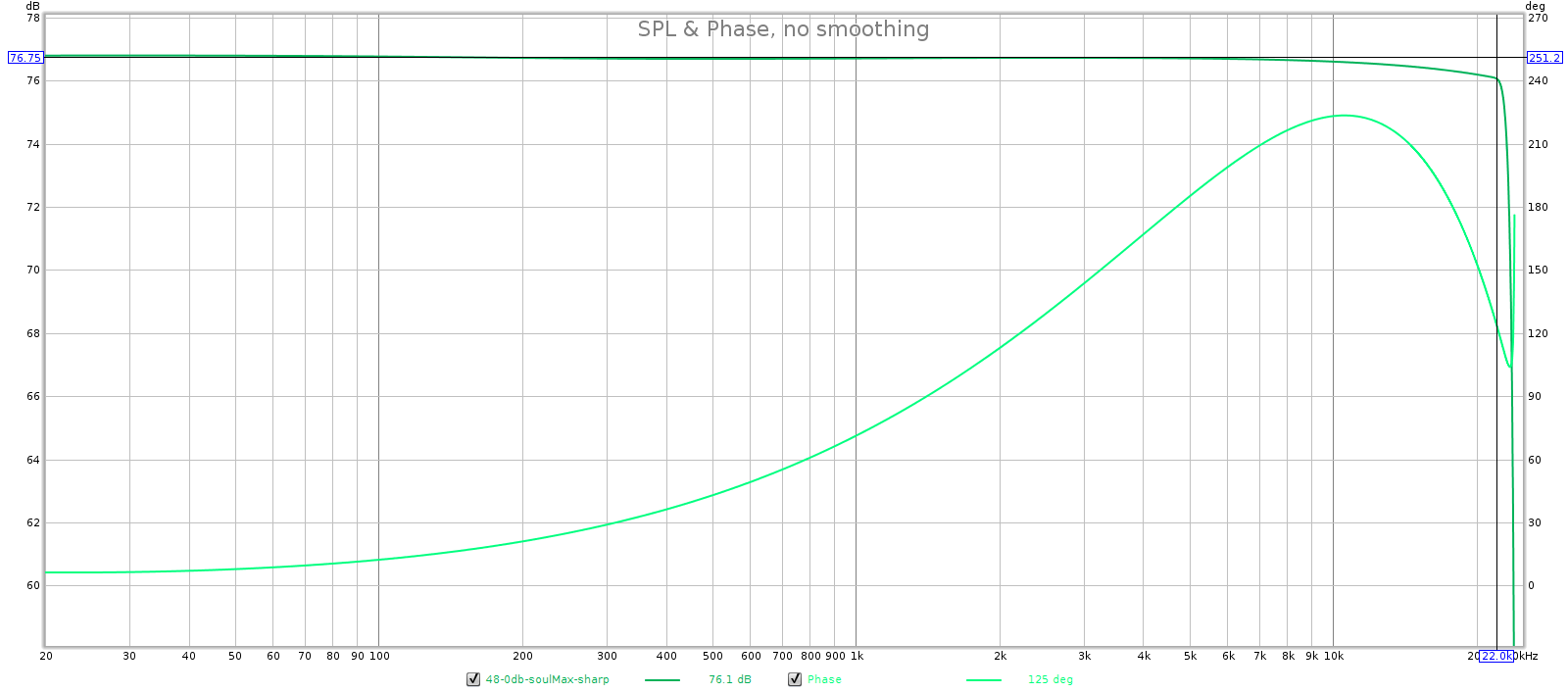
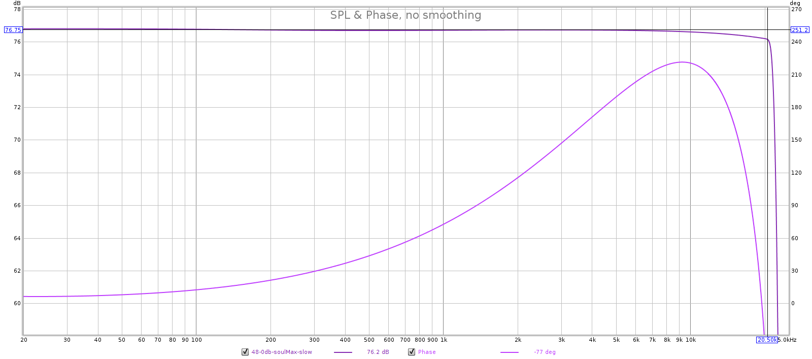
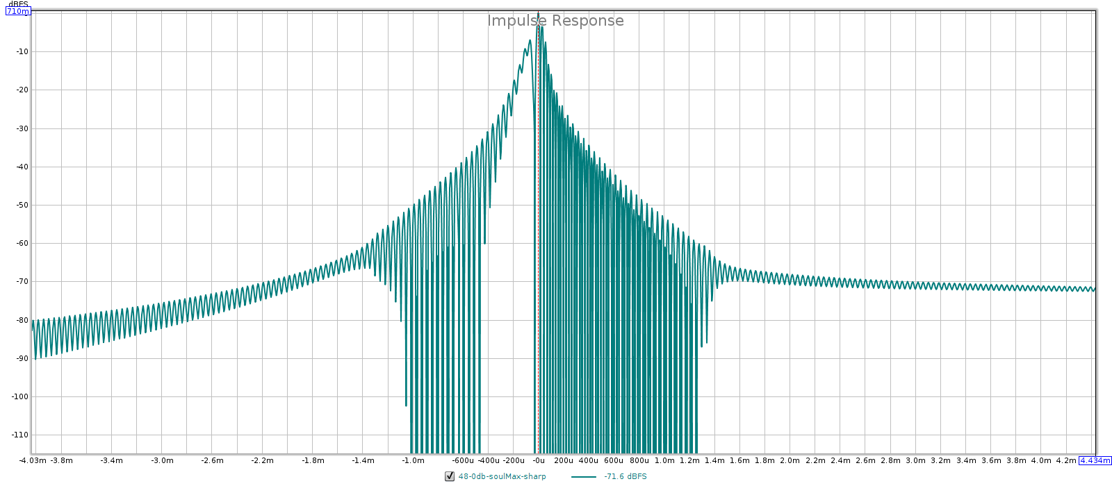
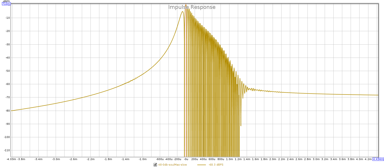
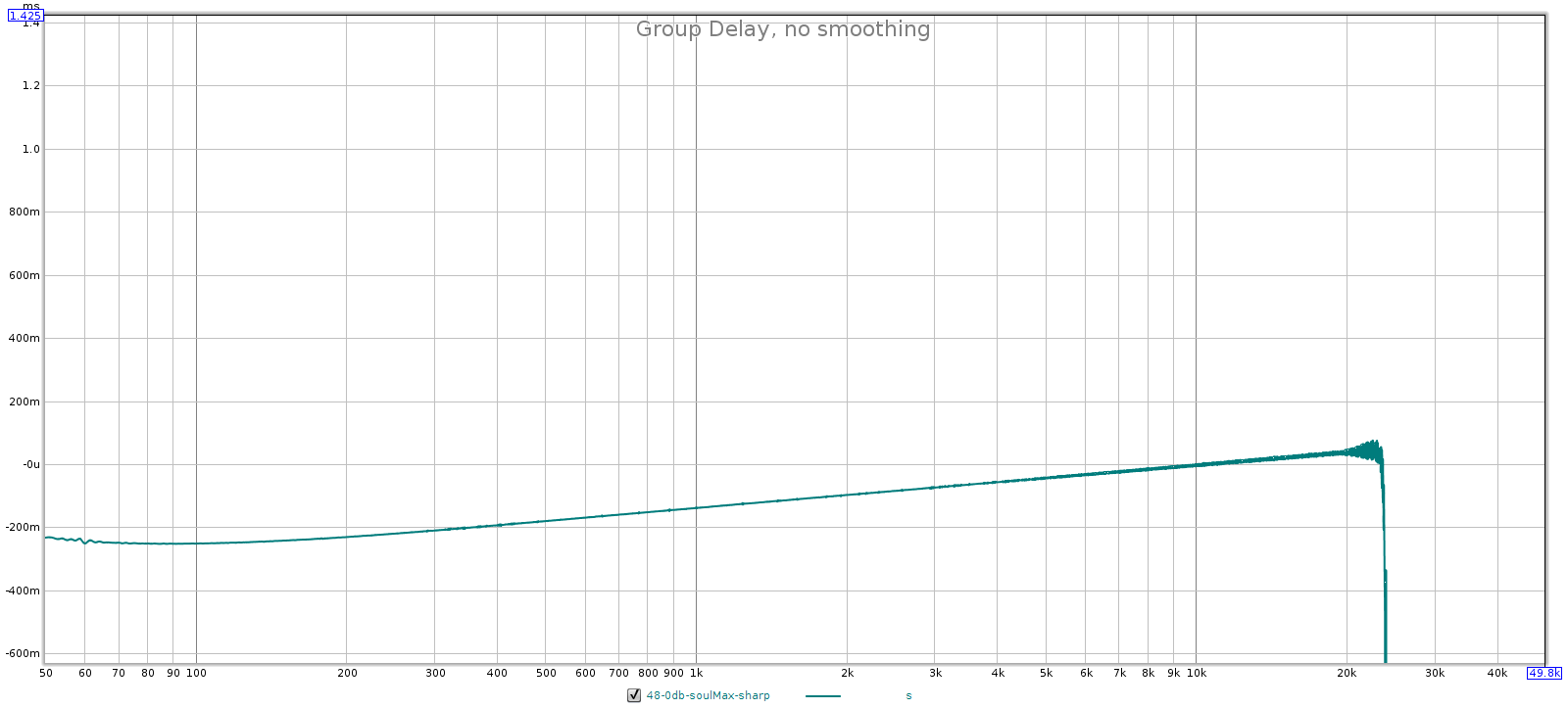
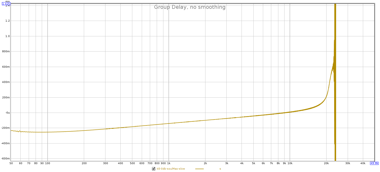
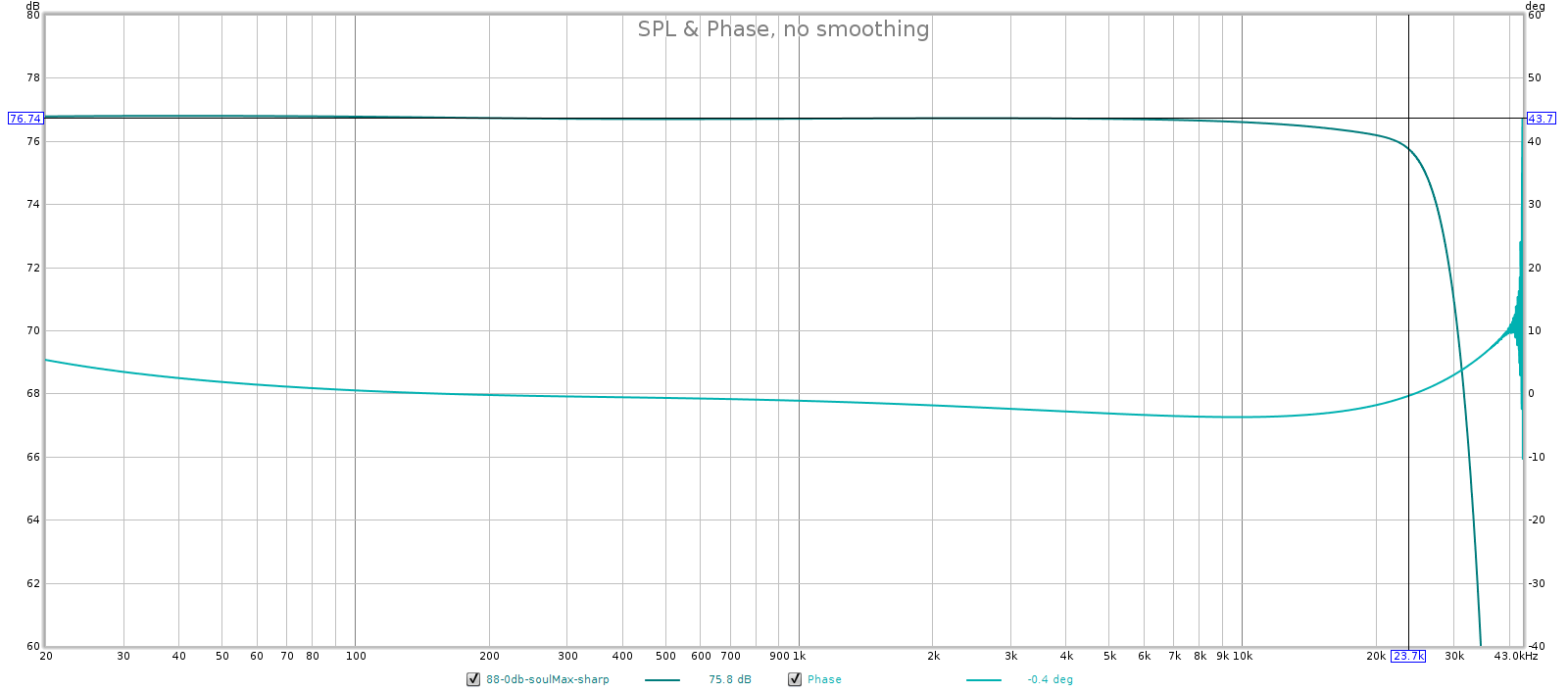
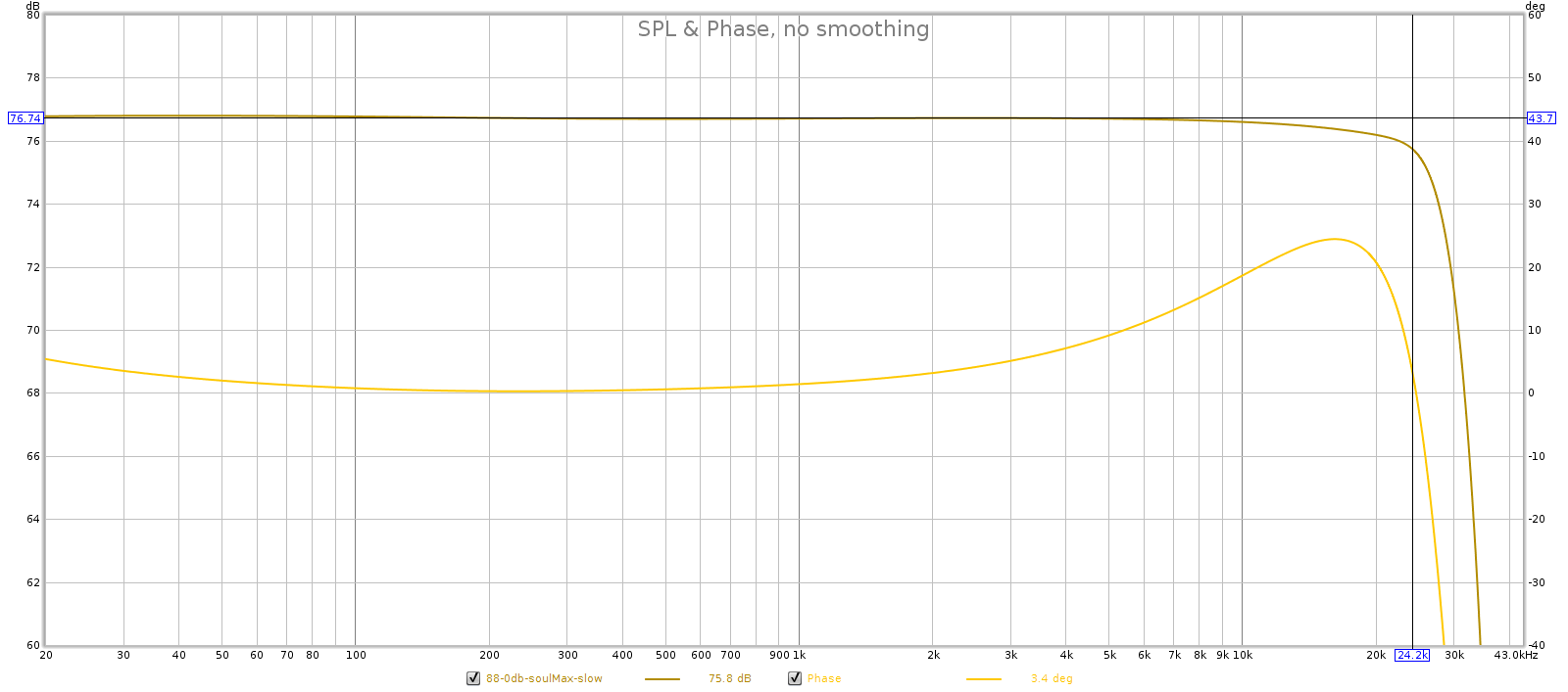
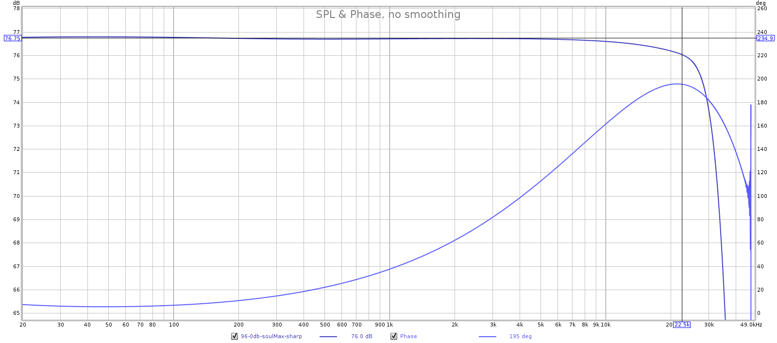
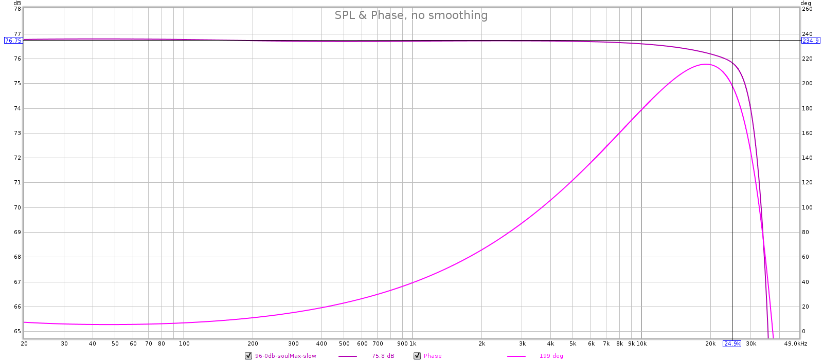
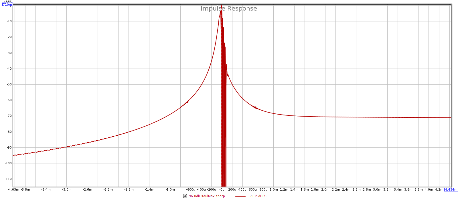
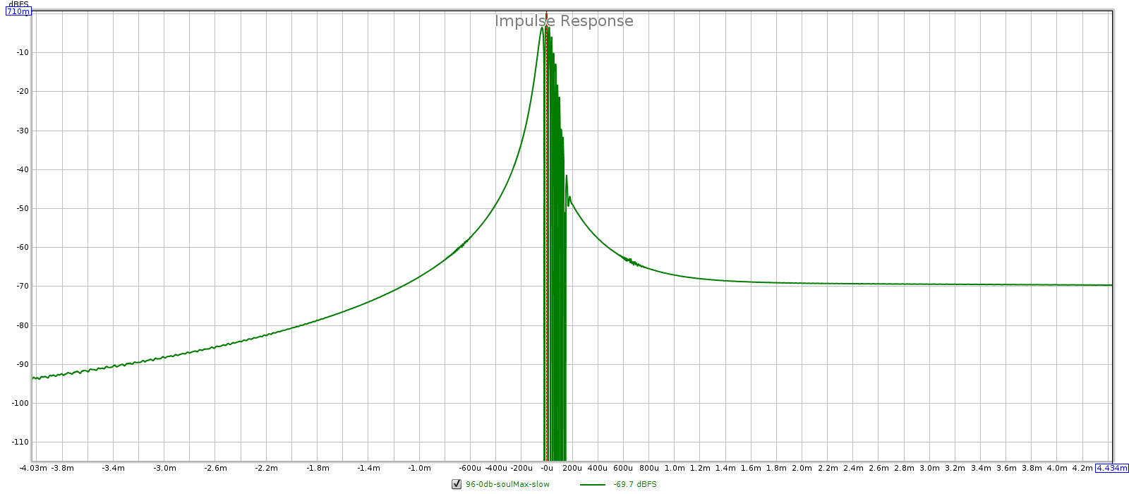
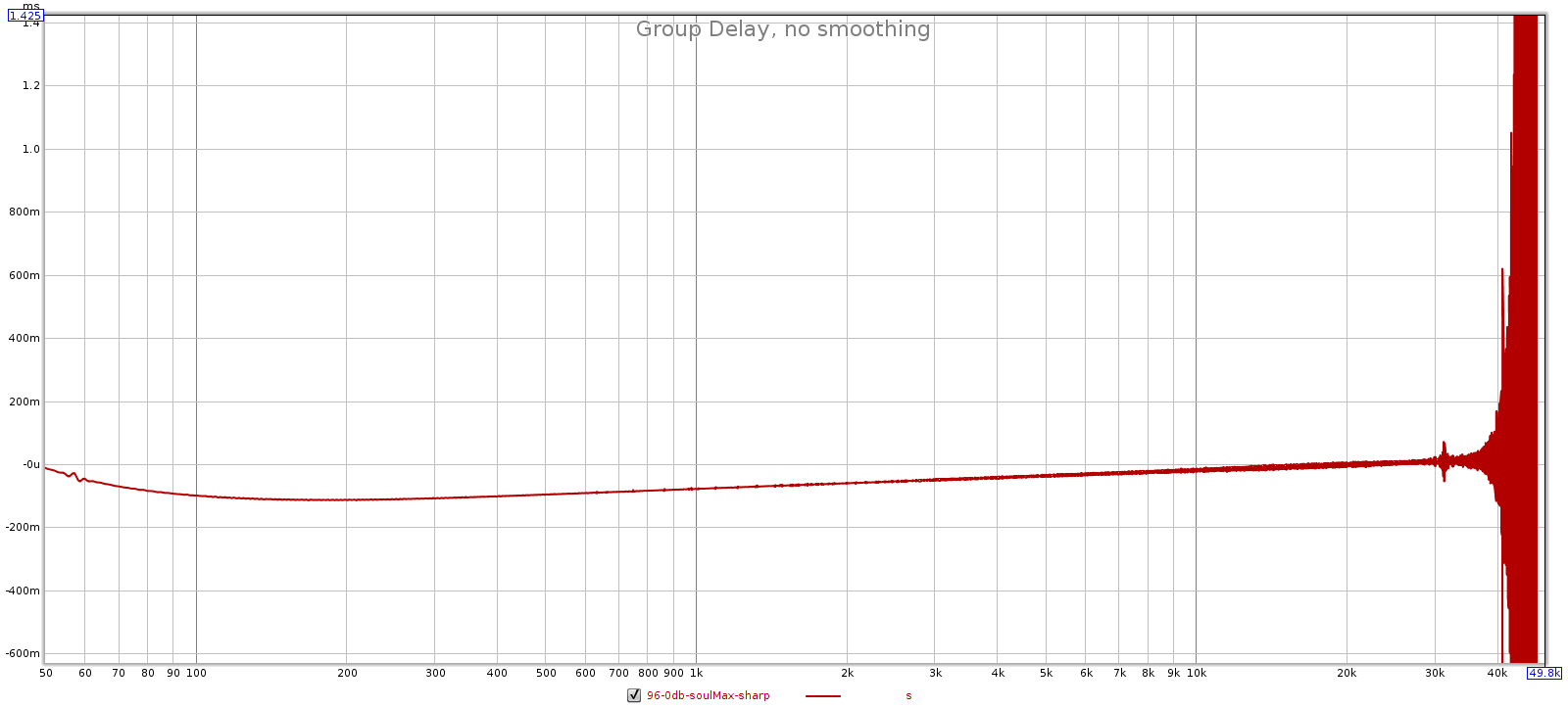
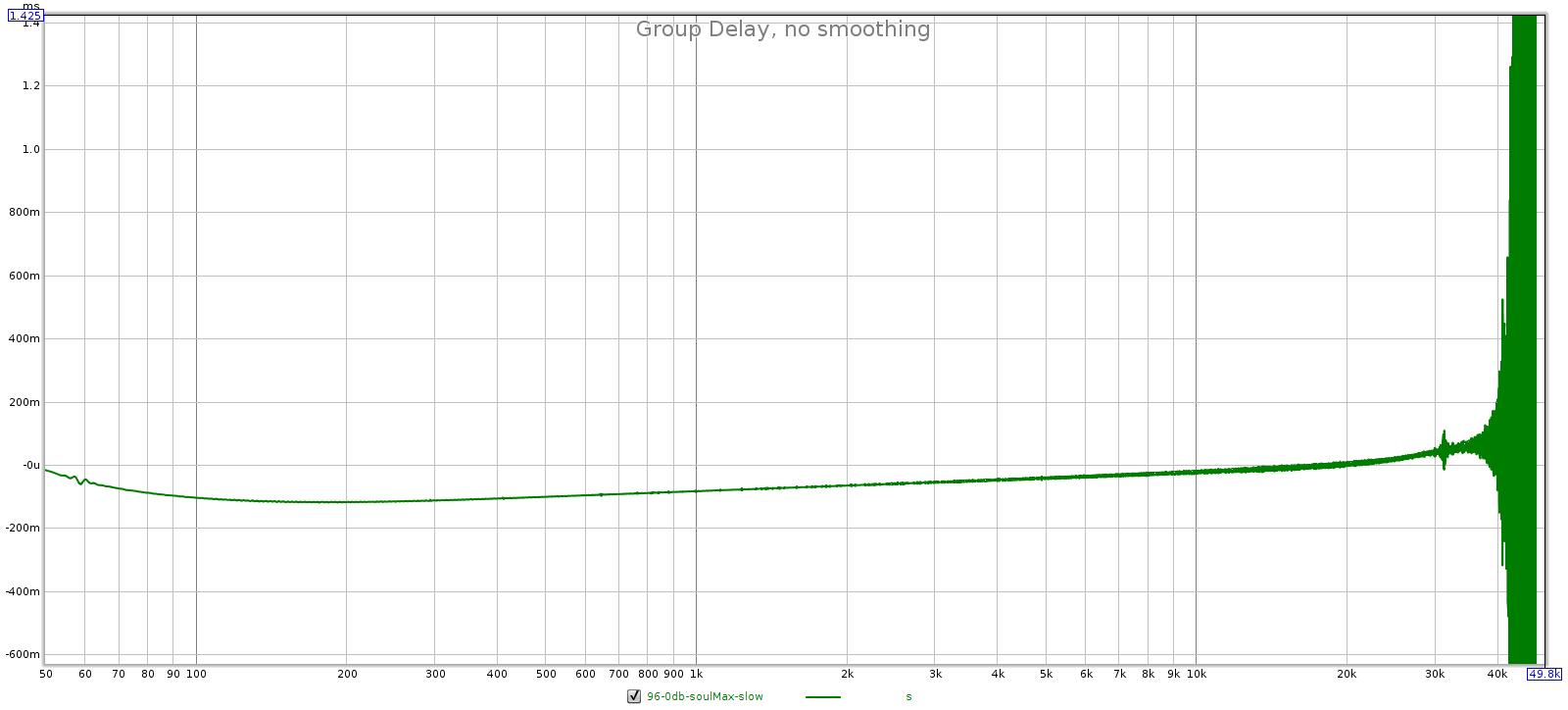
I measured the Soul’s output with the digital filter switch in each mode, sharp and slow, using 2 test signals: a frequency sweep and a square wave. From this, I measured frequency and phase response, group delay and impulse response. Charts/graphs are below, in the appendix.

Here’s the square wave: first sharp, then slow:

Overall, at 44.1 kHz I observed 3 key differences:

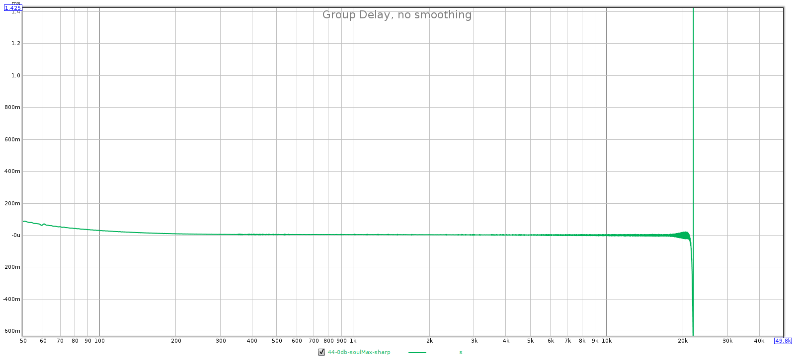
In sharp mode, frequency response and group delay are both flat to 20 kHz.
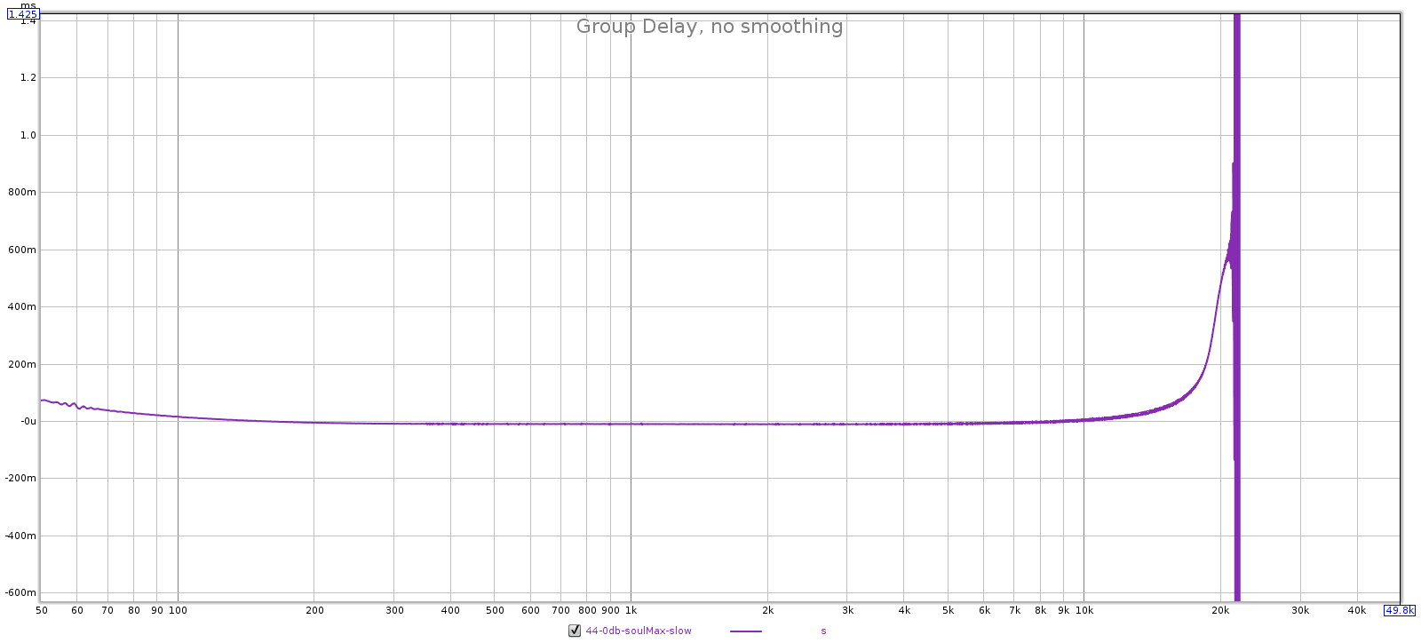
In slow mode, frequency response starts to roll off and group delay starts to rise between 18 and 19 kHz.
In slow mode, the square wave shows no ripple before a transition, and ripples with greater amplitude and longer duration after a transition.
The above curves are similar when comparing the sharp & slow filters at 48k sampling.

From these observations I conclude that for 44.1k and 48k signals, the Soul uses filters 3 and 4 in sharp and slow modes, respectively. Here’s why:

Because FR is flat to 20 kHz in sharp mode, it must be using filter 1 or 3.
Because GD is flat in sharp mode, it must be using filter 3.
Because FR rolls off just above 18k in slow mode, it must be using filter 2, 4 or 5.
Because GD rises in slow mode, it must be using filter 4.

Appendix

I recorded these graphs using my sound card, an ESI Juli@. This is not a great setup, but it’s the best I can do without dedicated equipment.

PC USB Audio output –> Corda Soul USB input –> Corda Soul analog output –> sound card analog input

Details:

Configured the sound card for analog balanced input & output (flip its daughter board from unbalanced to balanced.
Cabled from Soul to Juli@, using 3-pin XLR to 1/4″ TRS.
On PC:
- Disable pulseaudio
- Use Room EQ Wizard (REQW) on PC, in ALSA mode
- Configure REQW
  - set desired sampling rate (44.1, 48, 88.1, 96)
  - set audio output to USB
  - set audio input to Juli@ analog
- Configure Corda Soul
  - Select USB audio input
  - Ensure all DSP disabled (knobs at 12:00)
  - Set volume as desired
    - measured at max: 0 dB
    - measured at 12:00; -16 dB; 34 clicks down
- Use REQW “Measure” function
- Confirm proper sampling rate light on Corda Soul

Important Note: My measurements depend as much on the Corda Soul as they do on the Juli@ sound card. For example, if the Juli@ rolls off the frequency response faster than the Soul, then I will measure the same FR in both mods of the Soul. And if the Juli@ applies a minimum phase filter that adds phase distortion, then I will measure that phase distortion in both modes of the Soul. This probably explains why the digital filter responses were so similar at 88 and 96 kHz.

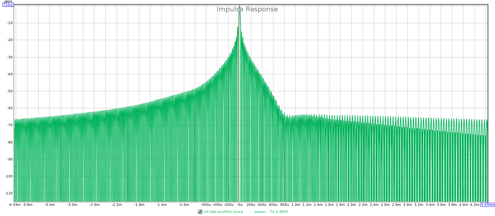
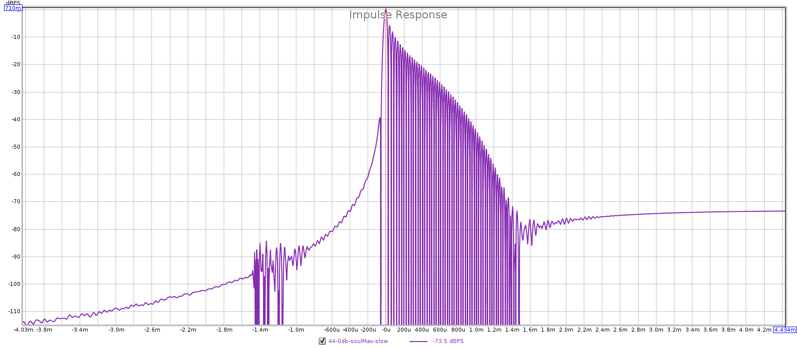
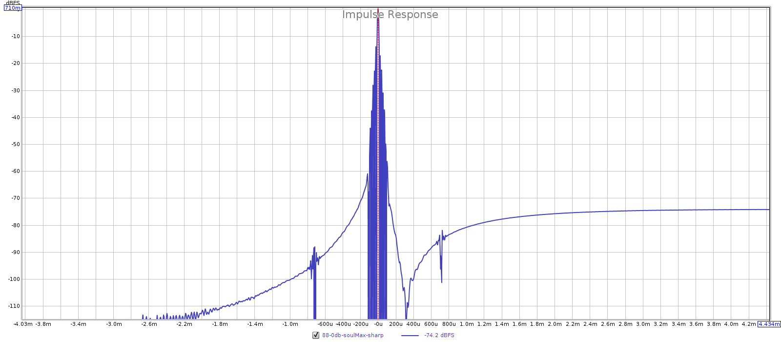
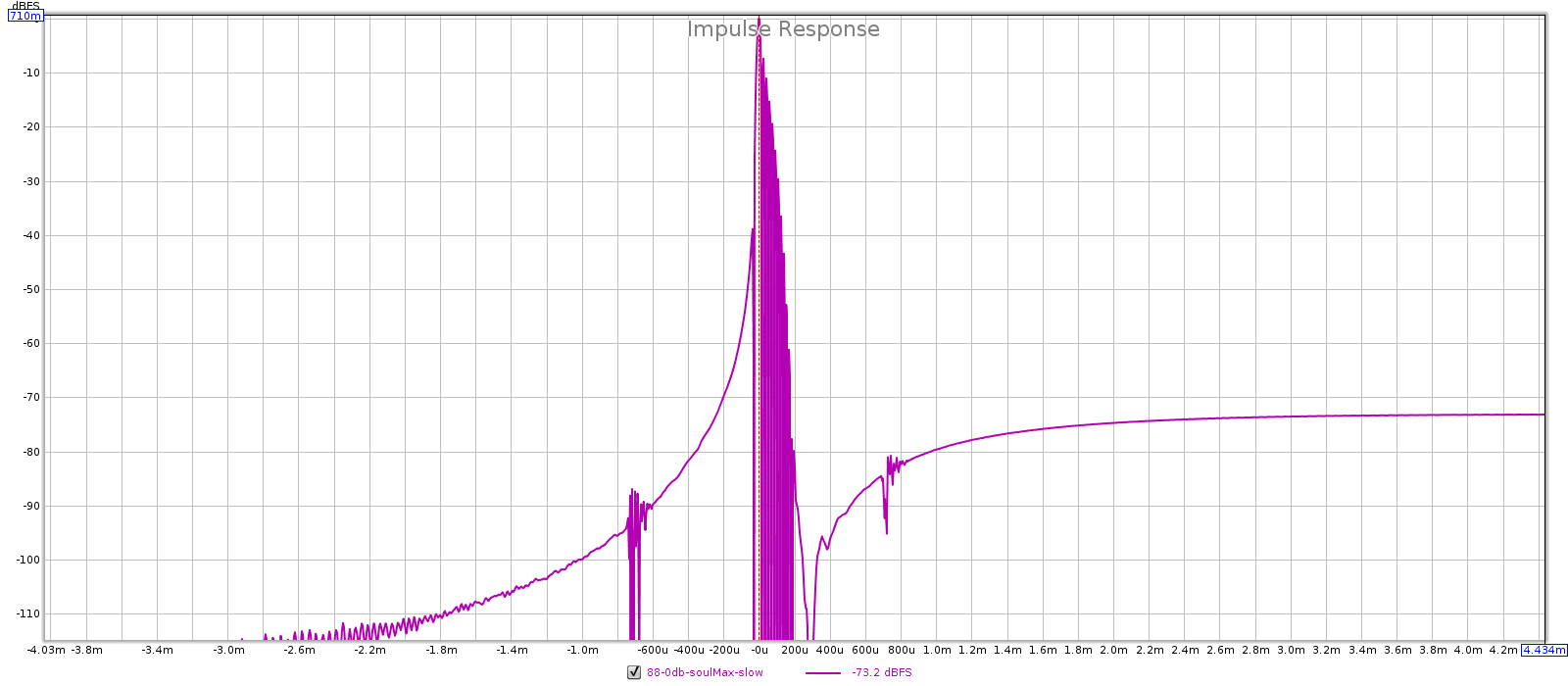
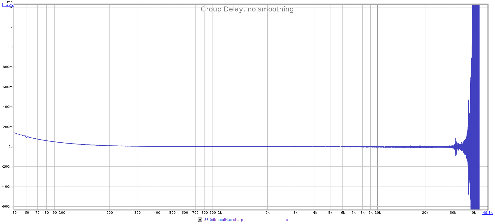
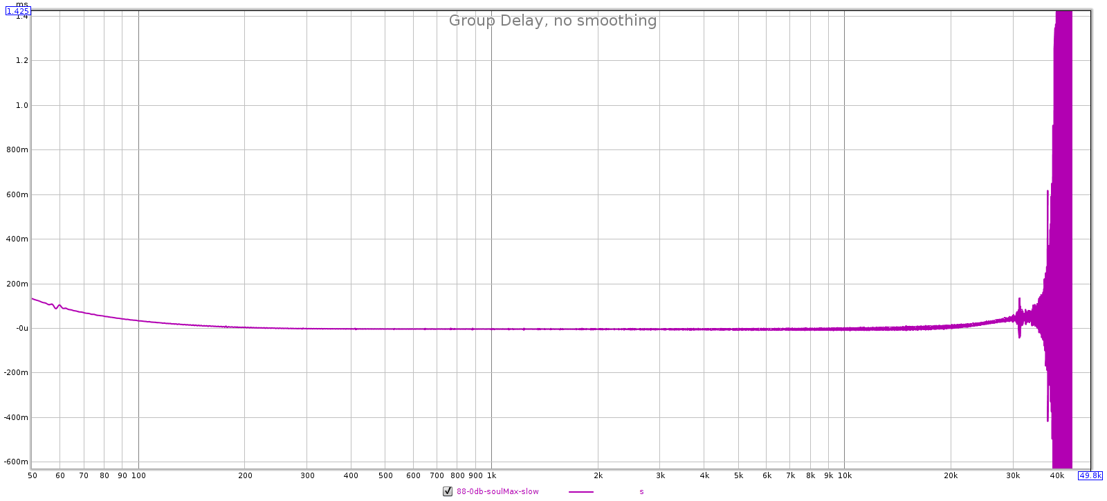
Here are FR, phase, GD and impulse plots for all tested sampling rates. Each is sharp top, slow bottom. Observe that at multiples of 44.1k (44.1k and 88.2k), the sharp filter has flat phase response while the slow filter does not. But at multiples of 48k (48k and 96k), both filters have similar non-flat phase response. This is probably due to the Juli@ card. However, the comments below assume the Juli@ card is transparent and all differences are due to the Soul.

In all cases, both filters at all sampling rates:

Frequency response: starts to taper at 20 kHz for the widest possible transition band.
Impulse response: sharp is symmetric, slow is asymmetric.
Group delay: sharp is flatter than slow.
At high sampling rates, the difference between the filters becomes immaterial. This is consistent with theory.

44.1 kHz: sharp is filter 3 and slow is filter 4.

Sharp FR doesn’t taper until past 20k, so it must be filter 1 or 3.
Sharp has flat GD, so it must be filter 3.
Slow FR tapers past 19k, so it must be filter 4 or 5.
Slow has more GD than sharp, so it must be filter 4.

48 kHz: sharp is filter 3 and slow is filter 4, for the same reasons as above.

88.2 kHz: Sharp is filter 2 and slow is filter 1.

Both FR start to taper at 20 kHz, so neither can be filter 3.
Both have a stopband at 44,100 kHz (beyond 40k), so neither can be filter 4 or 5.
Sharp has flatter phase / less group delay, which is filter 2.

96 kHz: Sharp is filter 2 and slow is filter 1.

Both FR start to taper at 20 kHz, so neither can be filter 3.
Both have a stopband at 48 kHz (beyond 44k), so neither can be filter 4 or 5.
Sharp has flatter phase / less group delay, which is filter 2.

Blind Audio Testing: A/B and A/B/X

November 22, 2019Audio, MathMike Clements
by Mike Clements

Blind Testing: Definitions

The goal of a blind audio test is to differentiate two sounds by listening alone with no other clues. Eliminating other clues ensures that any differences detected were due to sound alone and not to other factors.

A blind audio test (also called A/B) is one in which the person listening to the sounds A and B doesn’t know which is which. It may involve a person conducting the test who does know.

A double-blind audio test (also called A/B/X) is one in which neither the person listening, nor the person conducting the test, knows which is which.

In a blind test, it is possible for the test conductor to give clues or “tells” to the listener, whether directly or indirectly, knowingly or unknowingly. A double-blind test eliminates this possibility.

What is the Point?

The reason we do blind testing is because our listening/hearing perception is affected by other factors. Sighted listening, expectation bias, framing bias, etc. This is often subconscious. Blind testing eliminates these factors to tell us what we are actually hearing.

The goal of an A/B/X test is to differentiate two sounds by listening alone with no other clues. Key word: differentiate.

A blind test does not indicate preference.
A blind test does not indicate which is “better” or “worse”.
A blind test does not indicate what about the sounds is different, or why they are different – only whether they are.

Most people — especially audio objectivists — would say that if you pass the test, then you can hear the difference between the sounds. And if don’t, then you can’t. Alas, it is not that simple.

If you pass the test, it doesn’t necessarily mean you can hear the difference.
- You could get lucky: a false positive.
If you fail the test, it doesn’t necessarily mean you can’t hear the difference.
- You might tell them apart better than random guessing, but not often enough to meet the test threshold: a false negative.
If you can hear the difference, it doesn’t necessarily mean you’ll pass the test.
- False negative, like case (2).
If you can’t hear the difference, it doesn’t necessarily mean you’ll fail the test.
- False positive, like case(1).

Simply put, the odds are that if you pass the test, you can hear a difference, and if you fail, you can’t. But exceptions to this rule do happen, how frequently depends on the test conditions. Even a blind squirrel sometimes finds a nut!

Hearing is Unique

Hearing is quite different from touch or sight in an important way that is critical to blind audio testing. If I gave you two similar objects and asked you to tell whether they are exactly identical, you can perceive and compare them both simultaneously. That is, you can view or touch both of them at the same time. But not with sound! If I gave you two audio recordings, you can’t listen to both simultaneously. You have to alternate back and forth, listening to one, then the other. In each case, you compare what you are actually hearing now, with your memory of what you were hearing a moment ago.

In short: audio testing requires an act of memory. Comparing 2 objects by sight and touch can be done with direct perception alone. But comparing 2 sounds requires both perception and memory.

Audio objectivists raise a common objection: “But surely, this makes no difference. It only requires a few seconds of short-term memory, which is near perfect.” This sounds reasonable, but evidence proves it wrong. In A/B/X testing, sensitivity is critically dependent on fast switching. Switching delays as short as 1/10 second reduce sensitivity, meaning it masks differences that are reliably detected with instantaneous switching. This shows that our echoic memory is quite poor. Instantaneous switching improves sensitivity, but it still requires an act of memory because even with instant switching you are still comparing what you are actually hearing, with your memory of what you were hearing a moment before.

This leaves us with the conundrum that the perceptual acuity of our hearing is better than our memory of it. We can’t always remember or articulate what we are hearing. Here, audio objectivists raise a common objection: “If you can’t articulate or remember the differences you hear, then how can they matter? They’re irrelevant.” Yet we know from numerous studies in psychology that perceptions we can’t articulate or remember can still affect us — for example subliminal advertising. Thus it is plausible, as testing with brief switching delays suggests, that we do hear differences we can’t articulate or remember.

If this seems overly abstract or metaphysical, relax. It plays no role in the rest of this discussion, which is about statistics and confidence.

Accuracy, Precision, Recall

More definitions:

A false positive means the test said the listener could tell them apart, but he actually could not (maybe he was guessing, or just got lucky). Also called a Type I error.

A false negative means the test said the listener could not tell them apart, but he actually can (maybe he got tired or distracted). Also called a Type II error.

Accuracy is what % of the trials the listener got right. An accurate test is one that is rarely wrong.

Precision is what % of the test positives are true positives. High precision means the test doesn’t generate false positives (or does so only rarely). Also called specificity.

Recall is what % of the true positives pass the test. High recall means the test doesn’t generate false negatives (or does so only rarely). Also called sensitivity.

With these definitions, we can see that a test having high accuracy can have low precision (all its errors are false positives) or low recall (all its errors are false negatives), or it can have balanced precision and recall (its errors are a mix of false positives & negatives).

Computing Confidence

A blind audio test is typically a series of trials, in each of which the listener differentiates two sounds, A and B. Given that he got K out of N trials correct, and each trial has 2 choices (X is A or X is B), what is the probability that he could get that many correct by random guessing? Confidence is the inverse of that probability. For example, if the likelihood of guessing is 5% then confidence is 95%.

Confidence Formula

p = probability to guess right (1/2 or 50%)
n = # of trials – total
k = # of trials – successful

The formula:

(n choose k) * p^k * (1-p)^(n-k)

This gives the probability that random guessing would get exactly K of N trials correct. But since p = 1/2, (1-p) also = 1/2. So the formula can be simplified:

(n choose k) * p^n

Now, substituting for (n choose k), we have:

(n! * p^n) / (k! * (n-k)!)

However, this formula doesn’t give the % likelihood to pass the test by guessing. To get that, we must add them up.

For example, consider a test consisting of 8 trials using a decision threshold of 6 correct. To pass the test, one must get at least 6 right. That means scoring 6, 7 or 8. These scores are disjoint and mutually exclusive (each person gets a single score, so you can’t score both 6 and 7), so the probability of getting any of them is the sum of their individual probabilities. Use the above formula 3 times: to compute the probabilities for 6, then 7, then 8. Then sum these 3 numbers. That is the probability that someone will pass the test by randomly guessing to reach our decision threshold of 6. Put differently: how often people who are guessing will get at least 6 right.

Now you can do a little homework by plugging into this formula:

4 trials all correct is 93.8% confidence.
5 trials all correct is 96.9% confidence.
7 correct out of 8 trials (1 mistake) is 96.5% confidence.

The Heisen-Sound Uncertainty Principle

A blind audio test cannot be high precision and high recall at the same time.

Proof: the tradeoff between precision & recall is defined by the test’s confidence threshold. Clearly, we always set that threshold greater than 50%, otherwise the results are no better than random guessing. But how much more than 50% should we set it?

At first, intuition says to set it as high as possible. 95% is often used to validate statistical studies in a variety of fields (P-test at 5%). From the above definitions, the test’s confidence percentile is its precision, so we have only 5% chance for a false positive. That means we are ignoring (considering invalid) all tests with scores below 95%. For example, somebody scoring 80% on the test is considered invalid; we assume he couldn’t hear the difference. But he did better than random guessing! That means he’s more likely than not to have heard a difference, but it didn’t reach our high threshold for confidence. So clearly, with a 95% threshold there will be some people who did hear a difference yet our test says they didn’t. The test is wrong. Put differently, at 95% (or higher) we are likely to get some false negatives.

The only way to reduce these false negatives is to lower our confidence. The extreme case is to set confidence at 51% (or anything > 50%). Now we’ll give credit to the above fellow who scored 80% on the test. And a lot of other people. Yet this is our new problem. In reducing false negatives, we’ve increased false positives. Now someone who scores 51% on the test is considered valid, even though his score is low enough he was probably guessing (even if he doesn’t realize he was guessing).

The bottom line: the test will always have false positives and negatives. Reducing one increases the other.

Confidence vs. Raw Score

We said this above but it’s important to emphasize that confidence is not the same as raw test score. From the above, 7 of 8 is 96.5% confidence, yet 7/8 = 87.5%. In this case the raw score is 87.5% but the confidence is 96.5%.

If you get 60% of the trials correct, your confidence may be higher or lower than 60%. It depends on how many trials you did. The more trials you did, the more confident the 60% score becomes. For example, 3 of 5 is only 50% confidence; 6 of 10 is 62.3%; 12 of 20 is 74.8%. Getting 60% of the trials correct, you reach 95% confidence at 48 of 80, which is 95.4% confident.

The intuition behind this is that if you are doing only slightly better than guessing, consistency (more trials) is what separates random flukes from actual performance. If you flip a coin 6 times, you may frequently get 4 heads. But if you flip a coin 600 times, you will almost never get 400 heads. Put differently, you can sometimes win in Vegas, but you can’t consistently win else it would still be a desert.

Problem is, we’re limited in how many trials we can do. Listener fatigue sets in after 10 to 20 trials, skewing the results. You must take a break, relax the ears before continuing. So to get high sensitivity/recall from ABX testing requires multiple tests, in order to get high confidence from marginal raw scores.

Optimal Confidence

The ideal confidence threshold is whatever serves our test purposes. Higher is not always better. Lower is not always better. It depends on what we are testing, and why. Do we need high precision, or high recall? Two opposite extreme cases illustrate this:

High precision: 99% confidence
We want to know what audio artifacts are audible beyond any doubt.

Use case: We’re designing equipment to be as cheap as possible and don’t want to waste money making it more transparent than it has to be. It has to be at least good enough to eliminate the most obvious audible flaws and we’re willing to accept that it might not be entirely transparent to all listeners.

Use case: We’re debunking audio-fools and the burden of proof is on them to prove beyond any doubt that they really are hearing what they claim. We’re willing to accept that some might actually be hearing differences but can’t prove it (false negatives).

High recall: 75% confidence
We want to detect the minimum thresholds of hearing: what is the smallest difference that is likely to be audible?

Use case: We’re designing state-of-the-art equipment. We’re willing to over-engineer it if necessary to achieve that, but we don’t want to over-engineer it more than justified by testing probabilities.

Use case: Audio-fools are proving that they really can hear what they claim, and the burden of proof is on us to prove they can’t hear what they claim. We’re willing to accept that some might not actually be hearing the differences, as long as the probabilities are on their side however slightly (false positives).

Why wouldn’t we use 51% confidence? Theoretically we could. But there’s so much noise, our results become statistically meaningless. Using 75% reduces the noise (or false positives) while still recognizing raw scores only slightly better than random guessing, and using more trials to reduce false positives. For example, if our threshold raw score is 60%, we achieve 75% confidence at 15 of 25.

Conclusion

To mis-quote Churchill, “Blind testing is the worst form of audio testing, except for all the others.” Blind testing is an essential tool for audio engineering from hardware to software and other applications. For just one example, it’s played a crucial role in developing high quality codecs delivering the highest possible perceptual audio quality with the least bandwidth.

But blind testing is not perfectly sensitive, nor specific. It is easy to do it wrong and invalidate the results (not level matching, not choosing appropriate source material, ignoring listener training & fatigue). Even when done right it always has false positives or false negatives, usually both. We can adjust the confidence thresholds to adapt, but reducing false positives increases false negatives, and vice versa.

When performing blind testing we must keep our goals in mind to select appropriate confidence thresholds. High precision or specificity can be achieved in a single test, but high recall or sensitivity is harder, requiring aggregating results across multiple tests.

Corda Jazz: Measurements

October 8, 2019Audio, TechMike Clements
by Mike Clements

I own this headphone amp and use it every day at work. It has great sound quality with some unique features. I previously reviewed it and compared with other amps here.

Earlier this year I loaned this amp to Amir to measure for Audio Science Review, here. Amir does a great service to the audiophile community, I’ve met him in person and he’s a good guy with industry experience and a knowledgeable audiophile. However, we are all human with different opinions, and even objective measurements can be misleading.

Take SNR (signal:noise ratio) and SINAD (Signal over Noise and Distortion) for example. These are typically measured at a device’s full scale output, as this usually gives the highest number. But with headphone amps, we don’t listen at full volume. Their max output level is around 2-4 Vrms, sometimes more. This is far too loud for average listening levels; it would be painful or cause hearing damage. We typically listen with average levels around 70 or 80 dB SPL, which, perceptually, most people would describe as medium-loud. Most headphones reach this level with a voltage around 50 mV.

For example, consider the Matrix Audio Element, which Amir recently reviewed. It is one of the best DACs he’s ever measured, with a SINAD of 120 dB. However, its 50 mV SINAD is only 81 dB.

For comparison, The Corda Jazz measured about 87 dB SINAD at full output, and 90 dB at 50 mV output.

This illustrates an important point. We start with 2 devices. One has a SINAD of only 87 dB, which seems low. The other has a SINAD of 120 dB, which is the best he’s ever measured. Objective measurements tell us one is better! However, that is highly misleading because when you measure the output at levels we actually use, the exact opposite happens. The Jazz is actually 9 dB better than the Matrix. That’s a 65% drop in noise & distortion, which is a significant, audible improvement.

In short, the max SINAD measurement is correct, but misleading because it describes conditions that nobody actually uses when listening. The 50 mV SINAD is a better measurement because it represents actual listening conditions. But virtually nobody measures this; Amir (much to his credit) is the only person I know of who does this. Furthermore, the large variance between these two belies their similarity: as in the above example, the devices measuring the highest peak SINAD often do not measure the highest 50 mV SINAD, which proves how important it is to understand the measurements we make and their relevance to what we hear.

Enough said about this. Next I’ll talk about how the way an amp is designed affects this. If you don’t care about engineering details just skip to the conclusion.

Lesson learned: an amplifier’s SNR or SINAD can be quite different at 50 mV than it is at full output. How does this happen? The conventional amplifier has its internal gain-feedback loop set to whatever fixed gain ratio produces the desired maximum output, and the volume control is a potentiometer (variable resistor) that attenuates this. This “fixed gain with attenuation” means the noise level is relatively constant (based on the gain ratio, which is fixed), so as you turn the volume down, you reduce the SNR and SINAD at the same time.

This is easily seen with the Matrix. Full output is 3.9 V, so 50 mV is 38 dB quieter. And its 81 dB 50 mV SINAD is 39 dB less than 120 dB. What a coincidence: turn the volume down by 38 dB and SINAD drops by 39 dB! They have a virtually perfect 1:1 relationship. Not a coincidence; that’s by design.

So what’s happening with the Jazz? Its SINAD actually gets better at lower volumes. The Jazz is designed differently from typical amps. It does not use fixed gain with separate attenuation, but instead it uses variable gain to set the attenuation you need, obviating any need for separate attenuation.

The Jazz volume control changes the resistors in its internal gain-feedback loop. At low volumes, it has less gain and more negative feedback (wider bandwidth, lower noise and distortion). As you turn up the volume, you are increasing the gain (reducing negative feedback). [Incidentally, this means it must be inverting, for its gain-feedback loop to have less than unity gain. But its final fixed-gain stage is also inverting, so overall it does not invert.] Finally, this volume control is not a potentiometer; there is no potentiometer in the signal path.

This means the Jazz produces its best sound quality at the low to medium levels we actually use for listening. It also means the Jazz has perfect channel balance at every volume setting. Another observation from Amir’s measurements is that the Jazz is not current limited. It puts out 10x more power into 30 ohms, than 300 ohms.

Conclusion

Amir didn’t like the Jazz in his review, mainly because of its limited output power. One of the limitations of the Jazz’s unique volume control is that the resistors in the gain-feedback loop can only handle limited voltages. If you turn up the volume too high, it produces huge amounts of audible distortion due to input stage voltage clipping. The Jazz maximum output level before the onset of this clipping & distortion is about 3.7 V. That equates to 116 dB SPL with Sennheiser HD-580 and 120 dB on Audeze LCD-2. This is more than loud enough for me. Anyone listening this loud risks damaging his hearing. In fact, with the LCD-2 headphones I use the Jazz in low gain mode which is 16 dB quieter than this.

In summary, the Jazz is an amp that Amir’s measurements show has perfectly flat frequency response, perfect channel balance at all volume settings, less than 1 ohm output impedance (not current limited), and SINAD among the best he’s ever measured, at actual listening levels (50 mV). Yet he doesn’t recommend this amp because of its limited output voltage. At the same time, he does recommend amps like the Matrix, which have higher output power, but inferior measurements at the levels we actually listen. Amir is correct that exceeding an amp’s power limits creates audible distortion, thus is the most likely way listeners will hear distortion from an amp. However, if the limits are high enough (as with the Jazz), we won’t exceed them.

Put differently: it makes no sense to sacrifice sound quality at the moderate volume levels we actually use, in order to gain more power that we can’t use without damaging our hearing.

Classical Music Streaming: Primephonic & Idagio

September 28, 2019Audio, TechMike Clements
by Mike Clements

The Problem

Streaming classical music has 2 basic problems.

Note: I use the term “classical” in the most general sense, from ancient (pre-renaissance) to modern, including early music, baroque, classical, romantic, etc.

Fast forward 3 years and I'm now using Qobuz. I've added Qobuz to some of the comments below.

Metadata

ID3 has become the standard metadata for music, defining fields like title, artist, album, etc. This has an impedance mismatch with classical music. For example, if the Chicago Symphony is playing the Brahms violin concerto with conductor Reiner and soloist Heifetz, who is the artist? Brahms, Chicago Symphony, Reiner or Heifetz? What is the title? Violin Concerto in D Major, Opus 77, Chicago Symphony Live, or some nickname? If you search for this piece on streaming services like Spotify, Tidal, or Amazon, you will find all of the above, each individual recording having different metadata. Exacerbating this problem is the fact that every piece from every composer typically has tens if not hundreds of different recorded performances by different artists. This inconsistency makes it frustrating to find classical music.

Sound Quality

The sonic quality of the recording presents another problem. Most popular music is recorded with terrible sound quality: massive dynamic compression with clipping, and extreme amounts of EQ and other processing. They’re engineered to sound as loud as possible for radio, streaming and listening in noisy environments with crappy earbuds. This makes it easier for streaming, since the recording was already squashed to death by the studio during production, sound quality doesn’t matter because there’s nothing to preserve. However, sound quality matters with classical music. These recordings are made to a higher standard, having minimal studio processing, preserving dynamics and detail that lossy compression would destroy. This is important to reveal subtle variations in artistry, such as how a pianist voices chords, to a cello player’s bowing technique, to a flute player’s tone colors. This makes it harder to stream classical music.

So while there is plenty of classical music on standard streaming services, finding the piece you want, and the available recordings, is frustrating if not impossible. And when you finally do find it, listening to it through the streaming service’s lossy compression can be more disappointing than satisfying.

Thus it comes as no surprise that streaming accounts for only about 25% of classical music consumption, compared to 64% for the rest of the market.

The Solution

Even though classical makes up only about 3% of music sales, companies have formed to solve these problems. The 2 most popular are Idagio and Primephonic, and they address both of the above problems. I did not explore Naxos, because my experience owning about 100 of their CD recordings is that their sound quality (with a few notable exceptions) is second rate, and they only stream their own content, making great performances of the past inaccessible.

These classical music streaming services define and populate their own metadata customized for classical music, and they stream at lossless CD quality. This transforms the classical music streaming experience and has the potential to fundamentally change how music lovers experience classical music.

If that last statement sounds over the top, let me explain. With hundreds of composers, each writing hundreds of works, each having hundreds of recordings by different artists, each bringing something new to the artistic expression of the work, there is more classical music than any normal person can listen to in one lifetime. Of course, not all performances, nor all recordings, are equal. So music lovers have relied on reviewers to help sort through all of this. But reviewers and listeners are all people with different opinions. The work or recording a listener is interested in might not have been reviewed. When it has, a listener might find to his consternation that he disagrees with the reviewer. And many other works that a listener doesn’t even know about might be worth consideration. For decades, classical music listeners have relied on reviewers as gatekeepers and guides.

Streaming upends all of this by reducing to zero the marginal cost of the next recording you listen to. Browse the full catalog, using the classical music customized metadata to find works and performances in your area of interest. Take a chance on new works, recordings or artists, that the cost of individual CDs or downloads might have prevented you from listening to. Listen to everything and decide for yourself; the only constraint is your time. And, listen anywhere you are: home, work, in the car or wherever.

Furthermore, these streaming services cost less than a subscription to a classical music magazine like Grammophon or Fanfare. More on costs below.

Review

Idagio is a German company that’s about 4 years old. They are based in Berlin and their service became available in the USA about a year ago (September 2018).

Primephonic is a newcomer; their service started about a year ago (August 2018).

Both companies are staffed by a mix of musicians, musical scholars, agents and software engineers. They believe in what they’re doing and have the domain expertise to do it right.

I found many reviews of Idagio and Primephonic, but most were pretty shallow, as if the reviewers didn’t actually use the services in-depth on different devices and situations to discover their strengths & weaknesses. Since both services provide a 2-week free trial, I did this myself during a period where I did some business travel so I got their full experience from home, work, and traveling. Here is what I learned.

Getting Started

Both services offer a 14-day free trial. Primephonic is the quickest and easiest, since they don’t require a credit card. Just sign up with your email and it’s ready to go. Idagio requires a credit card to sign up for the trial, but they don’t bill anything to it until the 14th day.

Both services also let you sign up with a Facebook or Google account instead of using your email. I don’t do social media and prefer not to link online accounts, so I did not use this option.

Catalog

Their catalogs are roughly the same total size, and similar: both services had about 75% of the pieces I searched for, from early (pre-renaissance) music to modern. Where they differ, Primephonic has better coverage of early music, and less well known works and artists. Idagio has better coverage of baroque to modern classical music. For example, Idagio didn’t have some Piffaro (only 3 albums versus 6) and Joel Frederiksen early music albums that Primephonic had. Primephonic didn’t have Levin’s Mozart Requiem performance with the Violins du Roy, but Idagio did.

Some notable works were missing from both catalogs. Neither had anything from Jacqueline DuPre, nor did either have the Hillier Ensemble’s Age of Cathedrals (this is just one of several albums I have that was not in the catalogs of either service).

Addendum: Qobuz’s catalog is also fairly complete: with very few exceptions, everything I could find on Idagio or Primephonic is on Qobuz.

Metadata and Search

They both have metadata customized for classical music. You can search by any keyword, from composer to work to group, to album. And the search results are cross-referenced, so if you find a work, for example, you can click on it to see all other works from that composer, or all albums having that work.

I found their metadata doesn’t have much information about the album. For example if I search for “Liszt Transcendental Etudes”, they both show a list of albums. If I click on one, say Berezovsky (available in both), it shows me a picture of the album cover and says, “1996 Teldec Classics”. But there is no catalog number or other recording info, not to mention liner notes.

Both Idagio & Primephonic have the album booklets in PDF format for many albums (but not all). Primephonic has them more often than Idagio, and Primephonic makes them available in the mobile app as well as the browser, in contrast to Idagio which makes them available only in the browser. Coverage is gradually increasing with both services.

Primephonic’s search may not be quite as robust as Idagio. I searched for the Brahms Piano Quintet Op 34 in both. Idagio showed several recordings of it. It did not appear in Primephonic at all, as if they didn’t have this popular work in their catalog. When I mentioned this to Primephonic support, they sent me a link to the piece and said they would update their search. So they do indeed have it, but it wasn’t coming back in search results. But it did come back the next day, so they are listening to customers and actively improving their platform.

Addendum: Qobuz metadata is terrible. It’s not specific to classical music, but the same as other pop-oriented services like Spotify.

Music Discover-Ability

Despite this Primephonic glitch, in the Android app, their search is better than Idago’s. This is best explained by example. Suppose you want to find recordings of Liszt’s Transcendental Etudes.

In Primephonic: search for Liszt, tap him in results, and it shows a list of popular works. Tap Show All, but this list is too long to bother scrolling through, and you’re not sure whether it will appear under E for Etudes or T for Transcendental. The app has a Sort By box, enabling you to sort by Opus number, then you scroll to 139. Tap this, and it shows you 83 recordings which you can sort by popularity, A-Z, Z-A, newest, oldest, longest or shortest.

In Idagio: search for Liszt, tap him in results, and it shows 3 tabs: Works, Recordings, Albums. The Works tab has no way to sort or sub-search, it’s unclear how it’s sorted, and the list is too long to scroll, so that’s not helpful. The Recordings tab can sort by Date, Most Popular, or Recently Added, none of which help you find the Transcendental Etudes, so that’s not helpful. The Albums tab can sort by year or alphabetically, so this is not helpful either.

In short: Idagios’s Android app lacks sub-search or sort, making it more difficult to find the pieces you’re looking for. It’s easier to find things in the Primephonic app.

However, Idagio’s web browser does better than their app. Here, when you tap Liszt, Works can be grouped by Keyboard, Secular, Chamber, etc. This makes it easier to find stuff, but sort is still only by popularity or alphabet, so it’s still not as good as Primephonic.

Addendum: Qobuz scores low marks in this area, due to their metadata.

Applications / Players

Both services are fully functional in a web browser, and in Android and iOS apps that are free to install (not including the subscription price) from the standard app stores. By fully functional I mean you can search the catalog and play music. I ran both services on my Browser (Chrome & Firefox on Ubuntu 16 and 18), phone (Galaxy Note 4 SM-N910T running LineageOS 16 / Android 9) and my tablet (Galaxy Tab S SM-T700 running LineageOS 14 / Android 7).

Primephonic audio had brief gaps or glitches every 10 seconds or so when playing from Firefox on my laptop (which makes listening impossible), but this didn’t happen from Chrome on the same laptop, nor did it happen in Firefox on my desktop. So this problem was probably Firefox, not Primephonic. Audio from both apps was seamless on my phone & tablet.

UPDATE: these audio glitches turned out to be caused by Pulseaudio. Idagio streams at lossless CD quality which Pulseaudio handled just fine. Primephonic streams at higher than CD quality which was causing buffer under-runs in Pulseaudio. I reconfigured Pulseaudio to increase audio buffering and this made Primephonic glitch-free at all audio rates up to 192-24.

Idagio is more reliable with faster, smoother performance in both the browser and the Android app. Primephonic occasionally hung (both the app, and the web page) and had to be restarted or reloaded, which Idagio never did. Also, Primephonic had a bug in which the app’s streaming quality settings don’t appear to be saved, but revert to the defaults every time I saw them, even after I changed them.

UPDATE: as of June 2020, Primephonic has fixed these bugs in their app.

The Primephonic app supports both portrait & landscape mode, which makes it easier to use on my tablet. This is a nice little touch compared to Idagio’s app, which is always in portrait mode, even on the tablet.

Both apps enable you to download tracks or entire albums to your device so you can play them back anytime, even when disconnected. This was great on a cross-country flight. However, neither app supports external SD cards, so whatever you download consumes internal storage. When downloading, Idagio’s app creates an Android notification with a progress bar, and it also indicates in your music library the pending download status. Primephonic’s download is more of a black box – it doesn’t have a notification and you’re never sure exactly when it’s downloading, or when it might finish. But it does mark which tracks or albums in your library are downloaded, when complete.

UPDATE: as of June 2020, Primephonic app downloads give status notifications like Idagio.

Both apps stream smoothly and seamlessly, whether live streaming or playing pre-downloaded content, listening on headphones plugged into the device, or over bluetooth in my car. And my car’s audio next/previous track controls also worked when playing music from the apps on my phone.

Addendum: Qobuz is excellent here. They have their own player clients for popular platforms (iOS, Android, Windows, Mac) but they also are the only music streaming service that fully supports standard browsers in full audio quality – all the others compress or resample music streamed to a browser. Qobuz also has an open API, so for example USB Audio Player Pro plays Qobuz natively bit-perfect, so if you have an Android device it becomes an ideal source to feed into your DAC.

Sound Quality

Both support CD quality streaming as FLAC, which uses lossless compression. Listening to them on my audio system, the sound quality of both services was as good (or bad) as the recordings themselves on CD. To test this, I configured each service to stream in CD quality, then found CDs in my collection in each service, and streamed it with the CD playing, and quick switching back and forth I found them indistinguishable. My audio system is quite transparent and I can distinguish 320 kbps MP3 from CDs in blind listening tests, so this test suggests that each service is streaming the audio stream as-is, without processing it.

Primephonic streams at higher than CD quality for titles that support it. Primephonic’s highest audio quality setting uses MPEG4-SLS which streams the lossless raw recording when network bandwidth supports it, and falls back to AAC lossy compression when it doesn’t. As of June 2020, roughly half the content I listen to on Primephonic streams at higher than CD quality. I’ve seen sample rates of 44.1k, 48k, 88.2k, 96k, 176.4k and 192k, so it appears that Primephonic is streaming whatever raw bits the record companies provide, without resampling or converting them.

Both services also support lower quality (lossy compression) streaming to reduce data usage, which is useful for phones. These still offer good sound quality (192-320 kbps) that exceeds most other music streaming services.

Primephonic has settings for different rates on mobile versus Wifi data, which is useful and distinguishes it from Idagio, which just has a single quality setting.

Primephonic has gapless playback, but Idagio does not. Frequently, classical tracks or movements blend right into each other without any break in the music. Without gapless playback, the audio system inserts a break. This could be an important consideration for some listeners.

Qobuz is excellent here. They stream exactly what the studios or music rights owners give them, bit perfect. No resampling, lossy compression, or other processing.

Data Consumption

I mentioned that both apps can stream audio at true CD quality, yet they also provide lossy compression to save mobile data. This is especially useful because when listening on your phone, you’re often in a situation where reference quality audio isn’t needed: in the car or other noisy environment, using BlueTooth audio or earbuds plugged into your phone. Even some of the best IEMs and earbuds don’t have the same reference audio quality as full size headphones or listening rooms. So CD quality streaming only wastes mobile data when you can’t hear the difference.

I measured the actual data usage by each app when streaming audio over my mobile connection.

Before getting into the differences, here is approximate expected data usage per hour at a few standard music streaming rates:

128 kbps = 1 MB / minute, 60 MB / hour
320 kbps = 2.4 MB / minute, 144 MB / hour
CD (44 k / 16 b uncompressed) = 1,411 kbps = 10.5 MB / minute, 640 MB / hour
CD FLAC (lossless compression) = 6 MB / minute, 400 MB / hour
192-24 (the highest audio rate you’ll likely use)= 9,216 kbps = 69 MB / minute, 4.14 GB / hour

Primephonic

Offers 4 quality settings: Normal (128 kbps), High (256 kbps), Superior (320 kbps), Full (lossless up to 192-24). Also, allows different settings on WiFi versus mobile, which is quite useful.

However, when streaming music in the mobile app, Primephonic consumed about 200 MB per hour regardless of the setting. That is higher than 320 kbps. This is a bug in their Android app that makes it essentially unusable for streaming over mobile.

Update: As of June 2020, Primephonic has fixed this bug.

Idagio

Offers 3 quality settings: Normal (AAC 192 kbps), High (MP3 320 kbps), Lossless (FLAC of 1411 kbps). This is a single global setting whether on WiFi or mobile. It also offers a quality setting for downloads: Normal (750 Kb per minute, about 128 kbps), High (2.5 Mb per minute, about 320 kbps), or Lossless (up to 10 Mb per minute, but about 2/3 of that due to lossless compression).

When streaming music, Idagio consumed about 80 MB per hour at Normal and 200 MB per hour at High.

Customer Support

I emailed support for both services with various bug reports & suggestions. Both responded to all my emails, and not robotically but from an actual human who understood my message and gave a courteous, intelligent response. Primephonic was a bit faster, responding in less than 24 hours even on weekends. Idagio took a couple of days to respond, which is still quite good.

Addendum: Qobuz has great support. Every time I’ve emailed them I get a reply within 24 hours from a real human who understands the issue and is helpful.

Cost

Their cost is similar but not the same. Idagio is simple with a single service tier: $10 / month. No discount for buying a year up front, so it’s $120 / year.

Primephonic has tiered service depending on the streaming audio quality. It costs $10 / month for up to 320kbps lossy, and $15 / month for CD quality or higher. Primephonic has discounts for buying a year up front, which costs $100 and $150 respectively.

So, Primephonic can be the same price or more expensive than Idagio, depending on whether you want full CD quality streaming

Addendum: Qobuz used to be very expensive, but they lowered their prices a couple of years ago. They cost $11.90 / month all-in including taxes, or $143 / year.

Artist Reimbursement

Both services reimburse performers differently from other streaming services, in a way that is better suited to classical music, where track lengths vary tremendously. Reimbursing by track play starts just doesn’t make sense. Instead, they reimburse performers based on the time individual subscribers spend listening to specific tracks. In short, reimbursement is based on time spent, not starts.

Conclusion

To say that I’ve enjoyed these trials would be an understatement. It’s wonderful to have such a huge library of classical music at my disposal to listen wherever I want, at home, at work, in my car, or while traveling. Also, each service has curated lists of music in different areas of interest, which can be a useful exploration guide.

I like early music so I lean toward Primephonic due to their slightly better coverage, gapless playback, and their slightly better music search & discover-ability. However, the fact that their Android app always consumes 200 MB / hour when streaming is a show-stopper. And they’re more expensive, at least for full CD quality, and their app is a little more buggy.

I’m definitely going to subscribe to one of these services, but I still haven’t decided which one. They’re quite similar, each has its minor differences, pro & con, and neither is clearly better. I hope this detailed review has helped you decide whether you want a service like this and which might be best for you.

Addendum: after Apple acquired Primephonic, they only streamed to Apple devices, so I switched to Qobuz. The metadata is crappy for classical music, but I am enjoying the excellent sound quality and wide range of genres beyond just classical.

Magnepan/Dipole Speaker Setup

April 19, 2019AudioMike Clements
by Mike Clements

Having owned Magnepan 3.6/R for 20 years and set them up in 3 very different listening rooms, I’ve learned a few things. I want to capture the important things here.

Overview

Definitions:

Front wall: in front of the listener, behind the speakers.
Rear wall: behind the listener, in front of the speakers.
SBIR: speaker boundary interference response
- The total response at the listener position includes sound reflected from the front and side walls near the speaker.
- This response depends on the distance and angle of the speaker to these walls, and the treatment of those walls.
LBIR: listener boundary interference response
- The total response at the listener position includes sound reflected from the rear and side walls near the listener.
- This response depends on the distance and angle of the listener to these walls, and the treatment of those walls.
Speed of sound: 1130 f/s at sea level and 70*. Slower when cold, faster when warm.

All speakers are sensitive to room setup, but planars are dipoles which are more sensitive than conventional speakers. This is both a blessing and a curse. The blessing: if something isn’t right you can often fix it with simple rearrangement. The curse: for ideal sound, the speakers are going to be further into the room away from the walls.

SBIR

All speakers (even forward-firing cones) propagate both forward and back. But a dipole’s back wave has inverted amplitude.

Note: inverted amplitude is is often called or 180* out of phase, which is misleading. 180* out of phase means a shift, while inverted means a flip. Music has many frequencies superimposed so one wonders, 180* out of phase at what frequency? It is more precise to call it an amplitude inversion. More on this here.

Example 1: consider a speaker parallel to the front wall, 3′ away, which is 1/4 wavelength of 94 Hz. The back wave hits the front wall, reflects and as it passes the speaker it has traveled 1/2 wavelength, so it is 180* out of phase with the direct (non-reflected) wave from the speaker. This attenuates 94 Hz. But if the speaker is a dipole, it does the opposite (boosts) because the back wave started out with inverted amplitude, so shifting it 180* out of phase brings it back in-phase.

Conclusion: due to SBIR, dipoles boost the 1/4 wavelength frequency.

Example 2: consider what that same speaker does at 188 Hz (twice the frequency, half the wavelength). Now the 3′ distance is 1/2 wavelength, so the distance traveled is a full wavelength. A conventional speaker will boost this frequency because it’s in phase. A dipole will cut this frequency.

Conclusion: due to SBIR, dipoles cut the 1/2 wavelength frequency.

Direct vs. Reflected

Dipoles (electrostatic or planar magnetic) have a flatter impedance vs. frequency curve, without the strong Q resonances that conventional speakers have. This makes them a near-resistive load which is easy for amps to drive and gives them flatter phase response and group delay. I believe this contributes to their big, open, transparent sound relative to conventional speakers which can sound thick and muddy in comparison.

With all speakers, the sound you hear is a mix of direct and reflected. With dipoles this mix has relatively more reflected, less direct. This can make them sound big and phasey in underdamped rooms. With dipoles your room typically needs more damping than it does with conventional speakers.

One way to tackle this is to damp the walls to reduce reflection. How much damping you need and where to put it depends on the room size, shape, materials, and your personal preference. Too much damping and the dipole will sound thick & muddy like a conventional speaker.

Some dipoles (like Magnepans) have a rise in bass response that is supposed to be attenuated by the back wave reflected from the front wall. Because of this, they need to be the right distance from the front wall, and you don’t want to damp that wall too much.

Conclusion: in small to medium sized rooms, you will need to damp the wall behind dipoles to some extent, but not entirely. This damping must be effective down into bass frequencies, so it can’t just be acoustic foam; it must be tube traps, bass traps, etc.

LBIR

This topic doesn’t at first appear to be unique to dipoles, but it turns out to have an important difference. Consider a listener 3′ in front of the rear wall. Sound from the speakers reflects from the rear wall and comes forward, having traveled 6′ when it reaches the listener again. At 94 Hz, this is half a wavelength, so it attenuates that frequency. At 188 Hz this is a full wavelength, so it boosts that frequency.

What’s different about dipoles: the LBIR and SBIR distances, when equal, negate each other’s effects. With conventional speakers, they exaggerate each other. That is: if the speakers are 3′ from the front wall and the listener is 3′ from the back wall, the reflected waves don’t affect frequency response; SBIR cuts the same frequencies that LBIR boost. Conventional speakers give a double-sized cuts and boosts at the same frequencies.

Conclusion: when setting up dipoles in a small to medium sized rooms, try to make the LBIR and SBIR distances roughly equal. Put differently: the distance from the listener to the back wall should be the same as the distance from the speakers to the front wall.

Planar Speakers

March 15, 2019AudioMike Clements
by Mike Clements

More specifically, why I like planar magnetic speakers (and headphones!).

Sound quality: this one is subjective, yet important. When set up properly, planars sound more natural, open, and transparent than conventional speakers. They’re perfect for acoustic music across all genres from small to large ensemble classical, jazz, vocals, etc. Solo piano, vocals and chamber music are particularly good on planars. Their midrange is uncolored, having incredibly high resolution, yet without the artificial detail of boosted upper mids/treble, and without adding the glare or edginess of conventional dynamic drivers — unless that edginess is in the recording itself! With the 3.6/R I frequently hear subtle musical details or tone/balance shifts that I never hear even on the best headphones. Music is mostly midrange, and that is what planars do best. And the treble is simply astounding. No speaker on Earth matches the high frequency extension and linearity of those huge ribbon tweeters. The transition from the mid panel to treble ribbon is seamless, preserving the timbre and harmonic structure of acoustic instruments and voices. And that bass… clean, tight, with a seamless linear transition from the mids.

Low distortion: Measuring total distortion in Room EQ Wizard, my Magnepan 3.6/R measure about -60 dB (0.1%) in the treble, -50 dB (0.3%) in the midrange, and -40 dB (1%) in the bass (at 60 Hz). That’s lower than most conventional speakers, even lower than most headphones. And it is an uncorrected figure, including the distortion in the microphones, amplifier, and DAC; the actual distortion from the speakers alone is even lower. The Audeze LCD-2 headphones (planar magnetic) measure < 1% total distortion throughout the entire frequency spectrum, even to sub-bass frequencies. No conventional headphone matches that, not even the Sennheiser HD-800.

Why is planar distortion so low? I can think of 2 reasons. First, each Mag 3.6 panel spans the area of about six 12″ woofers, and its ribbon tweeter is 5′ long. Such physically large drivers take only very small movement/excursion to produce a given sound level. And the distortion that a driver produces is related to its excursion. Second, the drivers don’t have as strong Q resonances as conventional drivers do, both mechanical and electrical.

Linear phase: The 3.6/R have a relatively flat impedance curve: 4.2 ohms in the bass, to 3.3 ohms in the treble. They don’t have the big impedance vs. frequency swings that conventional speakers have. This promotes linear phase and flat group delay. The 3.6/R measure group delay of a flat zero through most of the frequency range, and only exceeds 10ms in the bass (below 80 Hz).

Easy load: Because planars have relatively flat impedance vs. frequency, they are primarily resistive loads that are easy for amplifiers to drive, despite their lowish impedance.

Drawbacks

Planars are dipoles, so they radiate equal energy front and rear, and the rear energy has inverted phase. This makes them more sensitive to room setup than conventional speakers. This can be a blessing or a curse, depending on your situation.

Planars tend to be inefficient, so they require more power for the same listening level. However, their dispersion is line-source (rather than a point-source), so the volume does not drop with distance as quickly as with conventional speakers.

Planars have limited maximum loudness. In a medium-large listening room, the bass distortion of my 3.6/R begins to rise at 95-100 dB SPL (and requires 400+ watts per speaker to attain). This is plenty loud enough for me, but it’s not for those who listen at ear-shattering levels.

Planars are difficult to measure because near-field, you can’t “hear” all the drivers from a single microphone position. And far-field, what you measure is as much the room as it is the speakers.

Planar drivers are side by side (the panel and the ribbon tweeter). They can’t be aligned vertically like conventional speakers, so the midrange to treble timing and impulse response depends on the angle between the speakers & listener. More specifically, the speakers should be angled so the panels are about 2″ closer to the listener than the ribbon tweeters.

Planars usually require a big room, and sound best when placed well into the room away from the walls. This leads to a low wife-approval-factor, and requires a dedicated audio room.

While planars have taut, low distortion bass, they usually don’t reproduce the lowest octave. The larger ones, like the 3.6/R, are good down to about 30 Hz, and 25 Hz is clearly audible though attenuated, which is fine for most music. But if you want that room-shaking 20 Hz rumble for movies with explosions and such, you’ll need a subwoofer.

Meier Audio “FF” Frequency Adaptive Feedback

March 4, 2019AudioMike Clements
by Mike Clements

Meier Audio has a feature in their amps called “FF” or Frequency Adaptive Feedback. Jan Meier describes it here. His article is detailed yet long. I wrote this article to complement it to help in understanding.

Musical Hearing

When it comes to human perception of sound and music, all frequencies are not created equal. The ear is most sensitive to frequencies from around 600 to 3000 Hz. And, most music (at least voices and acoustic music) is concentrated in this range.

Consequently, this is the most critical range for reducing distortion. You probably cannot hear 1% (-40 dB) distortion at 60 Hz, but you can hear it at 2000 Hz.

Analogy: Dolby B and RIAA equalization

Readers with a few grey hairs remember cassette tapes and Dolby B noise reduction from the 1970s and 80s. Dolby B was brilliant in its simplicity. Tape hiss has a wide frequency spectrum but it’s most noticeable in the treble (this is where our hearing is most sensitive). If you cut the treble during playback, it reduces hiss but it also dulls the music. So when recording, boost the treble. Then during playback, cut the treble by the same amount you boosted it. You get the same hiss reduction without any reduction in treble, because you’re only cutting exactly what you boosted earlier. The music has flat frequency response and sounds cleaner with higher S/N ratio.

The RIAA curve does the same thing for LPs. The pre-emphasis equalization curve cuts the bass relative to the treble before cutting the record groove. This reduces the groove and needle excursion needed to handle low frequencies, reducing distortion and noise. On playback, the phono head amp applies the opposite de-emphasis equalization curve, restoring flat frequency response.

The main drawback to this is that boosting the treble when recording limits the dynamic range. You can only boost it so far, before it reaches peak levels and overloads. Boosting the treble may require you to reduce the overall recording level. Alternately, reducing the bass lowers the SNR of the bass. Yet it improves the SNR of the treble, and this is a desirable tradeoff since that is where our hearing is much more sensitive to it.

Amplifier Feedback

Solid state amplifiers have a negative feedback loop that reduces distortion, increases bandwidth, and increases stability. Contrary to what we may read in some audiophile circles, negative feedback is A GOOD THING.

What exactly is negative feedback? An opamp’s native or open loop response, gain-bandwidth curve or transfer function, is not linear in frequency or amplitude. So a portion of its output signal is inverted and fed back into the input, which offsets these non-linearities.

Furthermore, an opamp’s open loop response drops with frequency, around 20 dB per decade or 6 dB per octave. This means negative feedback contains much stronger low frequencies than high frequencies. We can quantify this. Human hearing from roughly 20 Hz to 20 kHz spans a frequency range of 1000:1, or about 3 decades. So negative feedback is roughly 60 dB stronger at 20 Hz, than at 20 kHz.

Fractional Octaves

February 17, 2019Audio, MathMike Clements
by Mike Clements

I’ve been working with parametric EQ settings lately; here’s a quick cheat sheet.

Overview

We perceive the frequencies of sounds logarithmically. Each doubling of frequency is an octave. Thus, the difference between 40 and 80 Hz sounds the same as the difference between 4000 and 8000 Hz. Even though the latter difference is 10 times greater, it sounds the same to us. This gives a range of audible frequencies between 9 to 10 octaves, which is much wider than the range of frequencies of light that we can see.

Ratios

Two frequencies 1 octave apart have a frequency ratio of 2:1; one has twice the frequency of the other. A half octave is halfway between them on a logarithmic scale. That is, some ratio R such that f1 * R * R = f2. Since f2 = 2 * f1, R is the square root of 2, or about 1.414. Sanity check: 40 * 1.414 = 56.6, and 56.6 * 1.414 = 80. Thus 56.6 Hz is a half-octave above 40, and a half-octave below 80. Even though 60 Hz is the arithmetic half-way point between 40 and 80 Hz, to our ears 56.6 sounds like the half-way point between them.

More generally, the ratio for the fractional octave 1/N, is 2^(1/N). Above, N=2 so the half-octave ratio is 1.414. If N=3 we have 1/3 octave ratio which is 2^(1/3) = 1.260. Here is a sequence taken to 4 significant figures:

1 octave = 2.000
3/4 octave = 1.682
1/2 octave = 1.414
1/3 octave = 1.260
1/4 octave = 1.189
1/5 octave = 1.149
1/6 octave = 1.122
1/7 octave = 1.104
1/8 octave = 1.091
1/9 octave = 1.080
1/10 octave = 1.072
1/11 octave = 1.065
1/12 octave = 1.059

The last is special because in western music there are 12 notes in an octave. With equal temperament tuning, every note has equally spaced frequency ratios. Thus the frequency ratio between any 2 notes is the 12th root of 2, which is 1.059:1. Every note is about 5.9% higher in frequency than the prior note.

Bandwidth with Q

Another way to express the frequency range or bandwidth of a parametric filter is Q. Narrow filters have big Q values, wide filters have small Q values. A filter 2 octaves wide (1 octave on each side of the center frequency) has Q = 2/3 = 0.667.

For a total bandwidth of N octaves (N/2 on each side of center frequency), the formula is:

Q = sqrt(2^N) / (2^N - 1)

Here are some example values. You can check them by plugging into the formula.

N=2, Q=0.667
N=1.5, Q=0.920
N=1, Q=1.414
N=2/3, Q=2.145
N=1/2, Q=2.871

Note that these N octave fractions are total width, which is twice the above table which shows octave on each side of the center frequency.

Gotchas

Whatever tool you’re using for this, make sure you know whether it expects total bandwidth around the center frequency, or bandwidth on each side. And make sure you know whether it expects frequency ranges as raw ratios, fractions of an octave, or Q.

For example, consider a center frequency of 1,000 Hz with Q=0.92. The total bandwidth is 1.5 octaves, which is 3/4 octave on each side of the center frequency. The frequency ratio will be 1.682:1 on each side, or 2.83:1 total. Thus, this filter will affect frequencies between 1000 / 1.682 = 595 Hz and 1000 * 1.682 = 1,682 Hz. The total range is 595 to 1682 Hz which has a ratio of 2.83:1.

Real-World Correction

The above formula comes straight from any textbook. But these Q factors may give wider ranges than expected, due to an assumption it makes. This assumption is that the range of the filter is where the peak amplitude (at its center) drops to half its value. So the filter is still taking effect at these edges. If you want the filter to taper to zero at the edges, you need to use a bigger Q value to get a narrower filter. Roughly speaking, this means multiply the Q value by 2.0.

For example consider a filter that is -4 dB at 3,000 Hz, 3/4 octave wide on each side. That is a ratio of 1.682:1, so this filter tapers to zero at 3,000 / 1.682 = 1,784 and 3,000 * 1.682 = 5,045 Hz. Total width is 1.5 octaves (5,045 / 1,784 = 2.83 = 2^1.5). The above formula says this is Q=0.92. But that will be a wider filter. It will reduce to half (roughly +2 dB) at 1,784 and 5,045 Hz. If you want it to taper to zero at these edged then use Q = 0.92 * 2.0 = 1.84.

Note: this is an approximate / rough guide.

Example

Suppose you are analyzing frequency response and see a peak between frequencies f1 and f2. You want to apply a parametric EQ at the center point that tapers to zero by f1 and f2.

First, find the logarithmic midpoint. Compute the ratio f2 / f1 and take its square root to get R. Multiple f1 by R, or divide f2 by R and you’ll have the logarithmic midpoint.

For example if f1 is 600 Hz and f2 is 1700 Hz, the ratio is 2.83:1, so R = sqrt(2.83) = 1.683. Double check our work: 600 * 1.683 = 1010 and 1010 * 1.683 = 1699. Close enough.

So 1,010 Hz is the logarithmic midpoint between 600 and 1700 Hz. We center our frequency here and we want it to taper to zero by 600, and 1700. That range is a ratio of 1.683 on each side, which in the above list is 3/4 octave, or Q=0.920. Multiply Q by 2.0 to get Q=1.84 since you want this filter to have no effect (taper to zero) at these 2 endpoint frequencies. So now we know the center frequency and width of our parametric EQ.

Room EQ Wizard – A Great Tool!

January 27, 2019AudioMike Clements
by Mike Clements

Today I learned how to use Room EQ Wizard to tune my audio room. I had already done room tuning on my own and was happy with the results. But REW enabled me to get it even better.

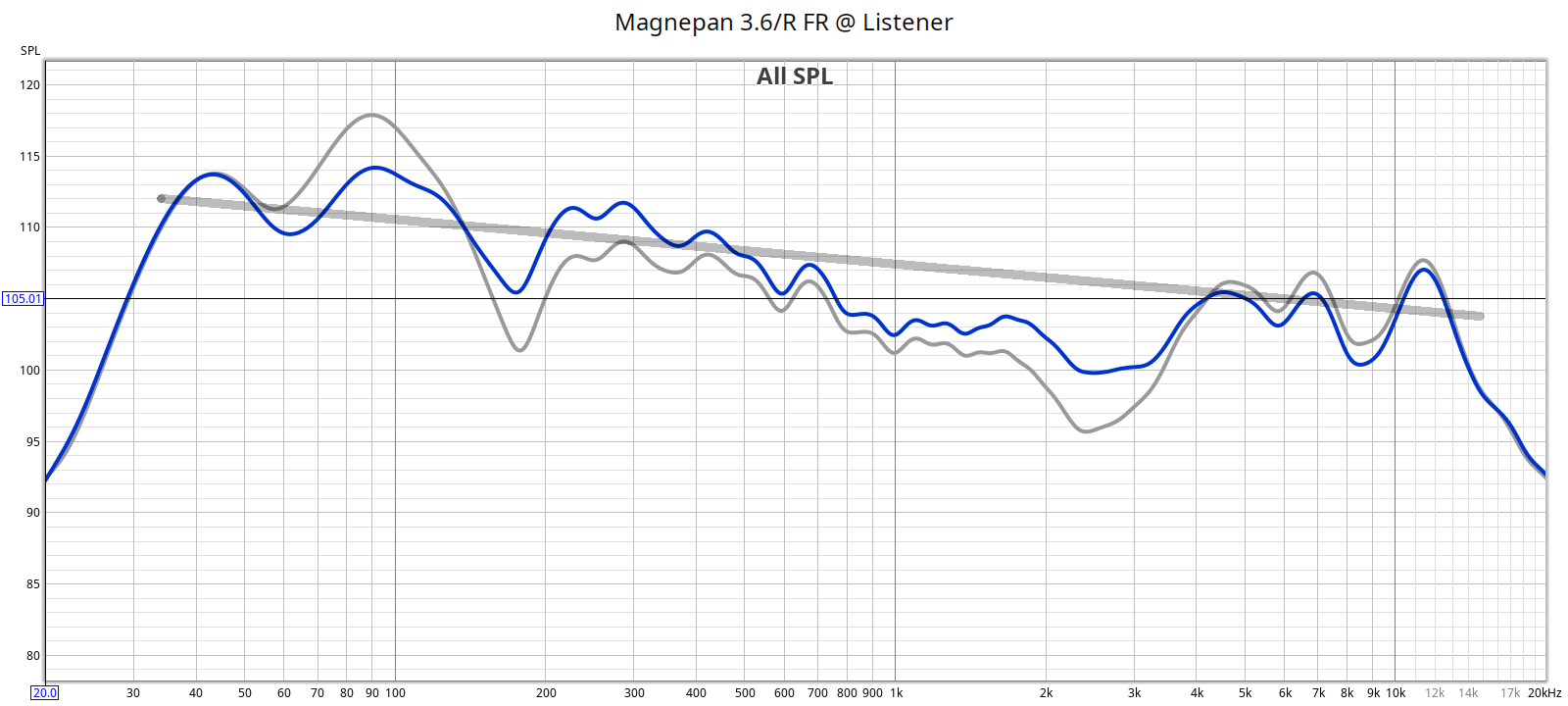
Here’s the final FR measured from the listener position, psychoacoustically smoothed (update: from Nov 2024). The Grey line is without EQ, the blue is with EQ. You can see that the EQ is only a few bands.

It’s linear and smooth, with a typical tapering response. This is a treated room having big tube traps, bass traps and acoustic foam. The parametric EQ is mild with gentle amplitudes and slopes. I’d rather have a few little bumps in the response, than perfectly flat response with bloated phasey sound from extreme EQ settings. Don’t let the cure be worse than the disease!

Overall, this smoothed response throughout the range. During test listening I can switch curves instantly while the music is playing. My ears like the difference, especially noticeable on good acoustic music recordings.

Caveat

Measuring from the listener position tells us what the speaker is actually doing, its in-room response, so long as the spatial response pattern of the microphone used to measure it matches the human head. You’re measuring the overall response which is a mix of the speaker’s on-axis (direct) and off-axis (reflected) response. The on-axis response is the most important part, yet this measurement doesn’t tell us whether the deviations (peaks or dips) come from the on-axis response, or from room reflections. If you fully EQ the deviations to flatten the overall response, you may be worsening the on-axis response and making the speaker sound worse – not better.

The takeaway is don’t go crazy with the EQ and fix every wiggle in the response. Room response measured from the listener position is a “result”, not a “target”.

Equipment & Details

Test audio files created by REW version 5.2 beta 4, burned to DVD-A
Oppo BDP-83 toslink PCM output
Behringer DEQ2496 digital EQ, toslink input and output
Corda Soul DAC-preamp, toslink input, XLR output
Adcom 5800 amp (28 years old), XLR input
Magnepan 3.6/R speakers (20 years old)
Room treatments (floor-ceiling tube traps, RPG acoustic foam, etc.)
MiniDSP UMK-1 measurement mic, and Rode NT1A mics, both calibrated
Recorded from the listener position

Here are the rest of the REW plots:

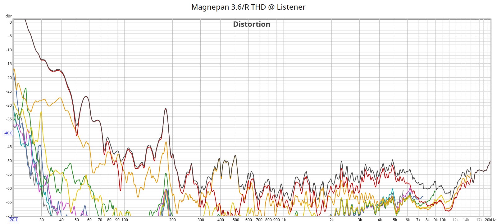
I measured distortion at the listener position and it includes all distortion from the power amp, microphone & recorder.

Total distortion is well below -40 dB (1%) above 70 Hz, and below -50 dB (0.3%) above 200 Hz. That is excellent for any speaker, even lower than most headphones. Distortion rises into low frequencies, which is common for speakers and not an issue since distortion is much harder to hear in low frequencies. The blip at 178 Hz is caused by room reflections, an SBIR null.

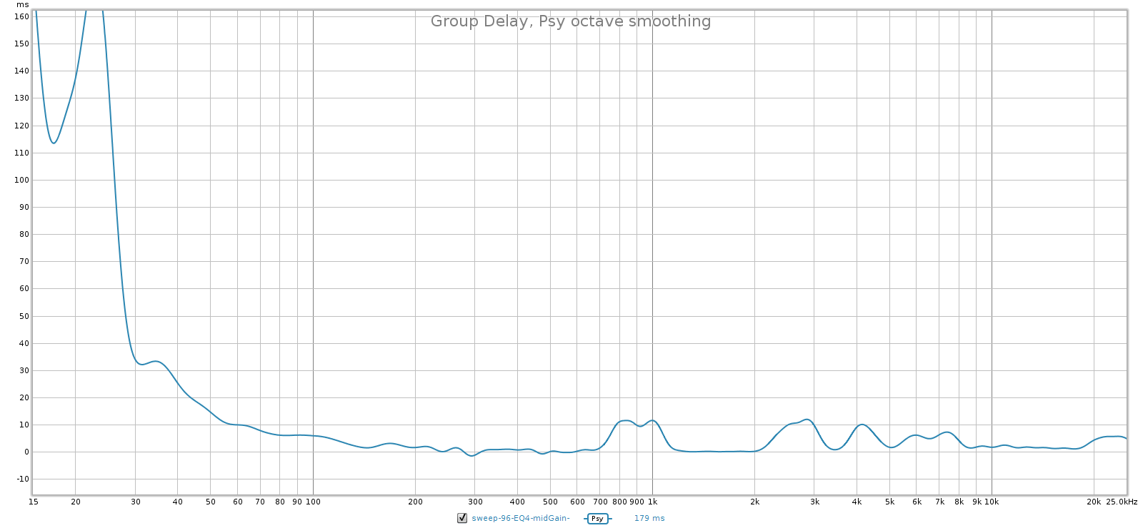
Group Delay is pretty flat. Rises in the bass as usual. But it’s 10 ms or less from 60 Hz on up, a near perfectly flat zero for most of the range. This seems typical of planar speakers.

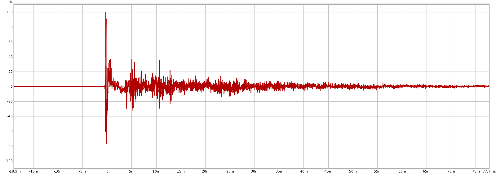
Initial impulse response is near zero in about 3 milliseconds, and you can see the reflections at 5 and 10 ms.

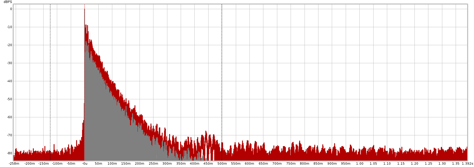
Total impulse energy is about -40 dB in the first 100 ms, from the listener position which includes room reverb. Room treatment damps the room, but it’s not completely dead. The grey is minimum phase IR, which is very close to the actual response.

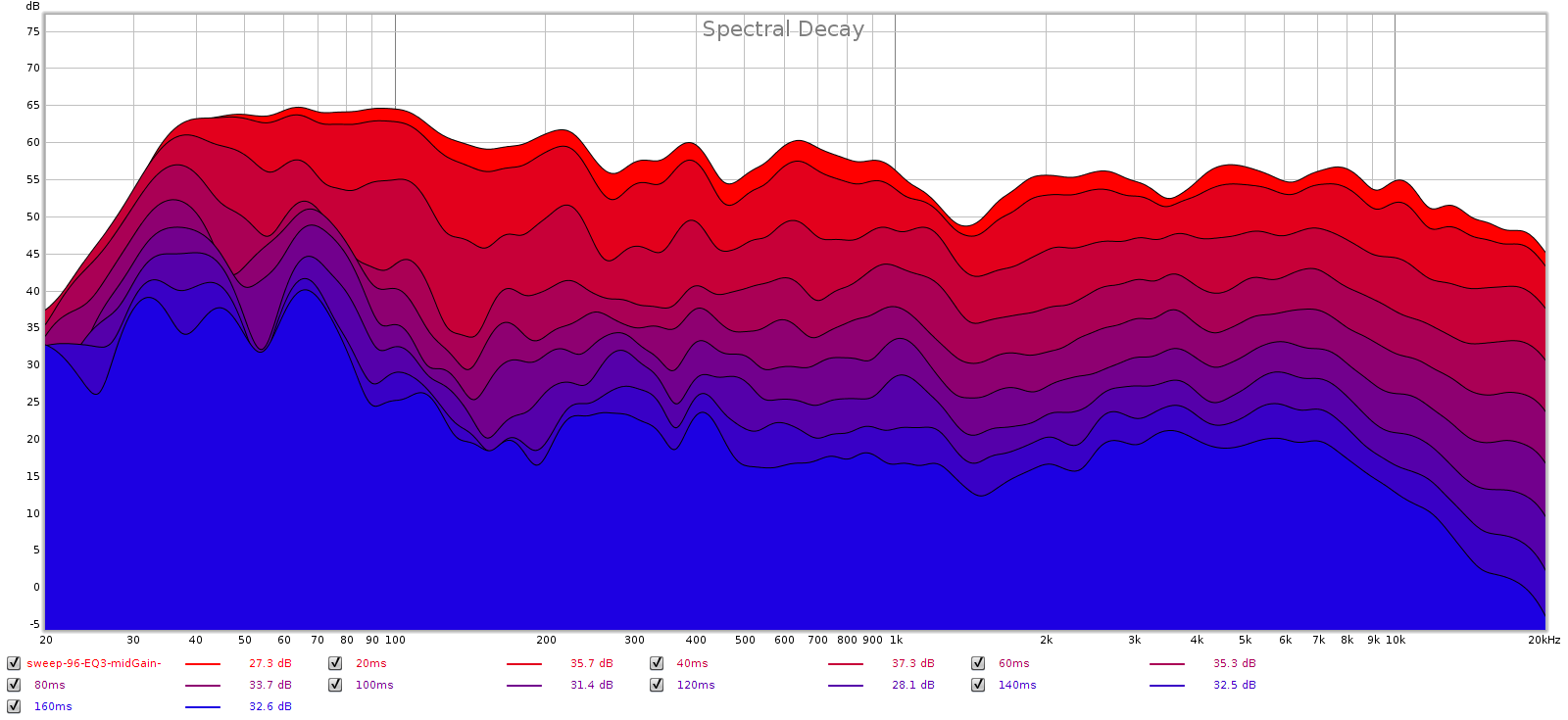
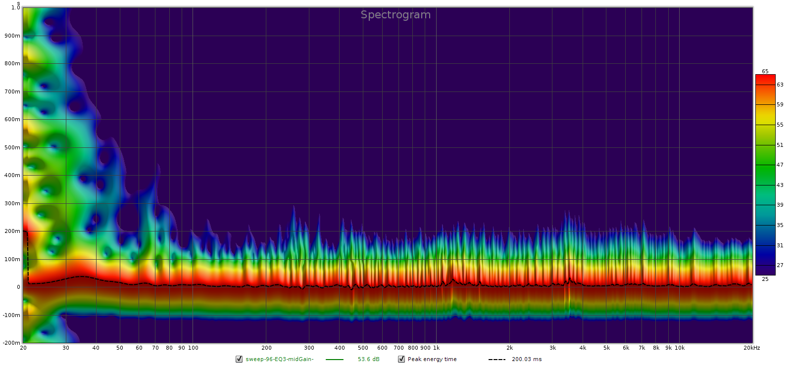
The CSD looks linear (no obvious ringing frequencies above the bass region) and decently fast. The room treatment certainly helps here:

Here’s the Spectrogram. There’s some mild ring around 64 Hz and rising decay time below 50 Hz. Overall pretty flat and even. That’s room treatments doing their job.

Since I treated this room I’ve been happy with the sound. With these measurements I was able to apply EQ to fine tune some things I couldn’t fix with room treatments.

Balanced vs. Unbalanced Conversion

January 10, 2019AudioMike Clements
by Mike Clements

Generally speaking, balanced and differential signaling are two different things. They’re often (but not always) used together, and in audio, the term “balanced” refers to this.

Speakers and Headphones

A speaker or headphone responds to the voltage difference between its 2 input wires. It doesn’t assume either is ground, though one might be, it doesn’t matter. So connecting a speaker or headphone to a balanced output is easy. Just wire (-) to (-) and (+) to (+) whether or not the (-) is a ground (unbalanced output) or carries a signal (balanced output). If the unbalanced output has a common ground for both channels (like a headphone), you can split it to both L and R (-) in parallel.

Converting a balanced speaker or headphone output to an unbalanced connector is not as simple. An unbalanced headphone cable (a standard 1/4″ or 1/8″) has 3 wires: L (+), R (+), and a single wire that is a common ground for the L and R. You can’t connect a balanced output’s (-) wires to this ground. That would mix the channels, and allow the amp’s output stages to drive each other, which is bad because they usually have very low output impedance, so it can overdrive the output stages. Also, you can’t just ignore the output’s (-) wires and connect the headphone (-) wires together; this will give a common floating ground. In short, you need a transformer to do this conversion.

Components

If the balanced/unbalanced conversion is between components like a preamp (not a speaker or headphone), it gets more complex because unbalanced components assume the (-) is a ground, but the balanced (-) carries a signal and its ground is a separate (3rd) wire. You can’t connect a balanced output (-) signal to ground; it will overdrive the balanced output as it tries to swing a voltage over a 0 ohm load. Also, you need to ensure the (-) wire has the same impedance to ground as the (+) wire.

So the best way to convert unbalanced to balanced between components is to use a transformer.

However, you can wire unbalanced output directly to balanced input. Connect the unbalanced (-) output to both pins 1 and 3 on the balanced side (negative & ground), and the unbalanced (+) output to pin 2 on the balanced side (positive). That is, carry the unbalanced source ground through to the balanced input. Since unbalanced (consumer) output is at a lower voltage than balanced (pro), the downstream balanced component will be receiving a lower level signal than it expects. This may or may not be a problem, depending on how clean is the input signal and the balanced device’s input voltage sensitivity and gain.