Category Archives: Tech

Slide Rules: Past the Basics

For background, here is part 1. It introduces slide rules and covers basic usage with C, D and CI scales. Here we cover the A, B and K scales for squares, square roots, cubes and cube roots.

A Scale: Squares and Square Roots

The A scale shows the square of each number on the D scale. Conversely, the D scale shows the square root of each number on the A scale.

Below the cursor shows that 3 on the D scale matches 9 on the A scale.

Note that as the D scale goes from 1 to 10, the A scale goes from 1 to 100. This means every single-digit number in the A scale has a corresponding double-digit number further up the scale. That is: 1 and 10, 2 and 20, 3 and 30, etc.

For example, below the cursor is on the A scale 30, showing the square root of 30 is 5.48:

So, squares are easy: just find the number on D scale and look to the corresponding number on A scale. But going the opposite direction, square roots, becomes ambiguous. What if you want the square root of a number that is not in the range of 1 to 100? For example:

  • If you want the square root of 400, on the A scale do you use 4 or 40?
  • If you want the square root of 4000,  on the A scale do you use 4 or 40?
  • If you want the square root of 0.5, on the A scale do you use 5 or 50?

First, observe that all of the single-digit numbers in the A scale occupy the first half, all the double-digit numbers the second half, and the split (the value 10) is exactly the mid-point of the scale. Thus, you can think of the A scale has having 2 halves. So the question boils down to knowing which half to use.

The answer is based on how many zeroes in the number whose root you want to know: is that number of zeroes odd or even? Adding or removing each zero (or each decimal point shift left or right) shifts back and forth between the 2 halves of the scale.

For example, consider the number 4.

  • The square root of 4 is 2 (low side of A scale).
  • The square root of 40 is 6.32 (high side of A scale).
  • The square root of 400 is 20 (low side of A scale).
  • The square root of 4000 is 63.2 (high side of A scale).

This pattern simply repeats. And it also repeats in the opposite direction:

  • The square root of 0.4 is 0.632 (high side of A scale).
  • The square root of 0.04 is 0.2 (low side of A scale).
  • The square root of 0.004 is 0.0632 (high side of A scale).

K Scale: Cubes and Cube Roots

The K scale works like the A scale. To cube any number N, find N on the D scale and look at the corresponding number on the K scale.

For example, this shows that 2 cubed is 8 (it actually shows that 2 squared is 4, and cubed is 8):

Yet the K scale also has the value 80, whose cube root is 4.31:

And the K scale also has the value 800, whose cube root is 9.28:

So while the A scale splits into 2 equal parts (1-10 and 10-100), the K scale splits into 3 equal parts: 1-10, 10-100, and 100-1000. Each of these occupies exactly 1/3 of the scale:

As with the A scale, cubing numbers is simple. Find N on the D scale and the corresponding K scale is N cubed. Yet doing the opposite, taking the cube root, is a bit more complex. You need to know which 1/3 of the scale to use. The procedure is a simple extension of what we did for the A scale. Yet since the A scale had only 2 parts, we thought of it as flipping back and forth. With the K scale having 3 parts, instead of flipping, each shift of the decimal point rotates forward to the next, or back to the prior part of the scale.

For example, consider the number 8:

  • The cube root of 8 is 2 (part 1 of  K scale).
  • The cube root of 80 is 4.31 (part 2 of K scale).
  • The cube root of 800 is 9.28 (part 3 of K scale).
  • The cube root of 8000 is 20 (part 1 of K scale).

It repeats every 3rd shift of the decimal point. And it also applies in the reverse direction as numbers get smaller:

  • The cube root of 0.8 is 0.928 (part 3 of K scale).
  • The cube root of 0.08 is 0.431 (part 2 of K scale).
  • The cube root of 0.008 is 0.2 (part 1 of K scale).

Exponents and Roots other than 2 or 3

Most everyday problems, especially those involving basic physics, use squares or cubes. Powers other than 2 or 3 are uncommon. Yet we do occasionally encounter them and you can solve them with a slide rule. The trick is to know some basic math rules about adding exponents.

Suppose we some number N, say 3.5, and we want to know N to some power, say the 7th power. So how would we compute 3.5^7 with our slide rule?

First, we split the exponent into smaller parts involving squares and cubes:

3.5^7 = 3.5^(2+2+3)

Next we split this out:

 3.5^(2+2+3) = 3.5^2 * 3.5^2 * 3.5^3

Now we have split the problem into squares and cubes so we can compute it on our slide rule:

3.5^2 = 12.2
3.5^3 = 42.8
12.2 * 12.2 * 42.8 = 150 * 42.8 = 6,430

Checking this with a calculator, I get 6,433.9. The slide rule gave us 3 significant figures.

Note: you can apply this same method with roots by taking the exponents as fractions. That is, the square root of 2 is 2 to the 1/2 power, cube root of 2 is 2 so the 1/3 power, etc.

What About that B Scale?

The B scale is the same as the A scale, used for squares and square roots. But it corresponds with the C scale instead of the D scale. Using D-A is the same as C-B. The B scale isn’t essential, but it is sometimes useful. On the Concise model 300, the A scale is along the outer circumference and the B scale is further inside. This makes the A scale longer and more accurate.

To quantify, on this Concise model 300 the A scale has a diameter of 9.2 cm and B scale 5.9. The A scale is 9.2 / 5.9 = 1.56 times longer. That’s a significant difference!

Conclusion

With squares and cubes, the power of the slide rule increases and we can solve a wider variety of problems. The next step is trigonometry: sine, cosine, tangent. These come up frequently in simple physics and everyday problems. This is covered in part 3.


Sanity Check: 0-60 Times

With electric cars, the classic performance metric of 0-60 time has gotten much faster, approaching the theoretical limits of available traction. Yet some cars show 0-60 times even faster than this, which seems impossible. Accelerating faster than available traction requires thrust that doesn’t depend on traction, like jet or rocket engines.

I suspect that the 0-60 times being quoted for some of these cars are not real, but just theoretical projections based on power to weight ratio. Here’s a way to sanity check them.

Braking is already traction limited. So when acceleration is also traction limited, the car should accelerate 0-60 in the same distance and time it takes to brake from 60-0. These might be slightly different, due to the car’s uneven front-rear weight distribution and different sized tires front and rear. But it’s still a good rough guide and sanity check.

Braking 60-0 is usually given as distance rather than time. But assuming constant acceleration (not exactly true but a decent approximation) it’s easy to convert. Remember our basic formulas:

v = a*t
d = 1/2 * a * t²

The best street legal tires have a maximum traction of about 1.1 G. You can get up to about 1.3 G with R compound racing tires, but most are not street legal and the ones that are, don’t last more than 1,000 miles.

Here’s how we compute this for 1.1 G with English units:

60 mph = 88 fps
1 G = 32 fps/s
v = a*t --> 88 = 32 * 1.1 * t --> t = 2.5 secs
d = 1/2 * a * t² --> d = 1/2 * 32 * 1.1 * 2.5² --> d = 110 feet

Braking from 60 to 0 at 1.1 G takes 2.5 seconds and 110 feet. If you look at the highest performance cars, this is about equal to their tested braking performance. So, that same car cannot accelerate 0-60 any faster than 2.5 seconds because no matter how much power it has, that is the limit of available traction.

Some cars claim to do 0-60 in 2 seconds flat. This is 1.375 G of acceleration and takes 88 feet of distance. It might be possible with R compound racing tires, but not with street tires. Any car that actually does this in the real world, must be able to brake 60-0 in 88 feet. If its 60-0 braking distance is longer than 88 feet, then it takes longer than 2 seconds to go 0-60.

Note: there’s rule of thumb for cars whose 0-60 time is power limited (not traction limited). Divide weight in lbs. by power in HP, then take half that number. For example, a 3,000 lb. car with 300 HP has a ratio of 10, and will do 0-60 in about 5 seconds. This of course is only a rough approximation, but it’s usually close; it works because acceleration depends on power to weight ratio.

Keyboards: Clickiez!

On a recent day at work my friend Joe dropped by with a new keyboard he built. “Try it out for a few hours” he said. It weighed half a ton and had an unusual layout, smaller than an 87-TKL 80% keyboard. I plugged in its standard USB cable and as soon as I hit a few keys my jaw hit the floor and a flood of nostalgia tickled my brain. I was back in the UC Davis computer lab in the 1980s on a VT-320 terminal connected to a PDP-11 running Unix. I had forgotten how much I loved those keyboards, even more than the buckling springs that my 4.77 MHz Leading Edge Model D, and most other PCs, had at the time.

Turns out Joe built that keyboard with Clickiez switches. They’re amazing!

They are rated at 40 grams actuation, but this is misleading because it’s not peak actuation force. I measured by stacking pennies on them and got 70-75 grams. This is the same as buckling springs or Cherry MX Greens, a bit heavier than normal clicky switches like Cherry or Gateron Blues. Clickiez makes a heavier version, but don’t bother. 40 grams sounds too light but it’s not really 40 grams and it’s perfect.

The sound is quite unique. Compared to Cherry or Gateron clicky switches, they’re quieter and lower pitched with more of a “thwock” than “click-tick”. The tactile feedback is far superior to anything made by Cherry or Gateron. Crisp, definite, solid and consistent. This is an unbeatable 1-2 punch. These are the best switches I’ve ever typed on.

These switches are compatible with Cherry and Gateron. Same physical dimensions, same pin-outs. You can get a hot-pluggable keyboard with Cherry or Gateron switches and swap them for Clickiez. However, each Clickiez switch top-case has a slightly different shape than Cherry or Gateron, which may conflict with some kinds of key stabilizers. I didn’t run into this, but beware.

Another unique aspect of these switches is they can be configured in 3 modes:

  • Clicky (default): medium force, crisp, tactile
  • Tactile: slightly heavier force, slightly quieter, less crisp, more tactile
  • Linear: lightest force, quietest, not clicky, not tactile

In addition, you can choose to lube them, or to use o-rings on the key-cap stems. Joe loaned me his leftover switches and I tried all combinations. I didn’t like the lube. Makes them just a tad lighter, quieter, softer and less crisp. It doesn’t seem like a big difference with a single switch, but when you do an entire keyboard, it’s huge – it completely transforms the feel. Some people might like it, especially if they’re used to laptop or bubble dome keyboards. The problem with lube is once applied, it’s virtually impossible to fully remove. So test it first! Key-cap o-rings make them a tad quieter with less harsh bottom-out and shorter stroke. No change in the weight or crispness. Tactile mode feels a bit wonky to me. I prefer the crispness of the default mode, and it’s plenty tactile.

NOTE: to reconfigure Clickiez switches you must pop open the switch case, remove & re-install the metal click-plate in a different position, then snap the switch case top back on. It helps to have 2.0x magnification, and before you reinstall the switch case top, gently bend the 4 snap prongs inward to ensure a snug fit.

I couldn’t resist – I had to have a keyboard with these switches! Joe recommended a DIY kit keyboard, but they were expensive. I love his custom-made half-ton keyboard with its thick slab of metal baseplate, but it’s not for me. For a daily driver I had to have something more conventional and budget-friendly. So I ordered a set of 90 Clickiez switches and bought a high quality hot-swappable 87-TKL layout keyboard with Gateron switches. Total cost for both was about $250. I pulled the Gaterons and installed the Clickiez in their default configuration.

Michelle had an old keyboard with Cherry Brown clone switches that was starting to die. I let Michelle try my new Clickiez keyboard. She loved it so I told her keep it, I’ll build another for myself. It also has the advantage of wired USB instead of wireless, which is simpler with superior response.

So I put in another order and built a second for work. I installed o-rings on the key-caps but it’s still a bit loud for typing on Zoom calls. As I type for extended periods of time, there’s no finger or hand fatigue. The o-rings help there, as they soften the bottom-out of the keys.

Note: I got a Keychron Alice layout keyboard for work, and added ZealPC V2 Zilent switches. These are a silent tactile switch, great for Zoom calls and not annoying your work neighbors. I use the Clickiez at home.

I still love buckling springs and use them at home. A while back I compared them to Cherry Blues: http://mclements.net/blogWP/index.php/2021/10/19/keyboards-cherry-blue-vs-buckling-springs

Compared to Clickiez, buckling springs are a smidge heavier in actuation and a lot louder with a very different timbre. The Clickiez are so different it’s hard to say which is better. Suffice to say Clickiez are the only switch that even comes close to buckling springs. Both are leagues ahead of anything from Cherry or Gateron. One advantage of hot-swap switch sockets is the modularity makes it a “forever” keyboard. If any switch ever fails, simply replace it. Can’t do that with buckling springs. Some have said the Clickiez are unique but not necessarily a daily driver kind of switch. I disagree and find them most excellent for all-day use.

References / links:

Clickiez switches: https://zealpc.net/products/clickiez
87-TKL Keyboard: https://mechanicalkeyboards.com/shop/index.php?l=product_detail&p=9270
Alice Keyboard: https://www.keychron.com/products/keychron-v10-alice-layout-qmk-custom-mechanical-keyboard

Corda COUNTry: All in One Audio

Summary

The Meier Audio Corda COUNTry is a unique little device:

  • Equalizer, headphone crossfeed, reverb and other audio functions implemented in DSP (Digital Signal Processing)
  • Inputs (digital only): USB, SPDIF coax and toslink
  • Digital outputs: SPDIF coax and toslink
  • D to A converter
  • Analog output: single ended RCA (line level, volume controlled)
  • Analog output: single ended 1/4″ headphone jack

Its purpose is to adjust or tailor the sound to listener preferences. You can use it in many ways, though they fall into 3 categories:

  1. Pure DSP upstream from your DAC
  2. Headphone amp
  3. Preamp

In the first case you already have a headphone amp or preamp and you only want the DSP features. In cases (2) and (3) the COUNTry is an all-in-one device. The COUNTry was originally designed for (1) without any D/A or analog outputs. Later, the D/A and analog outputs were added since they increase flexibility with minimal cost impact.

The COUNTry operates internally at a single fixed sample rate: either 96k or 192k (buyer’s option). Digital inputs are resampled (if necessary) to this rate. I received a 192k unit.

The COUNtry

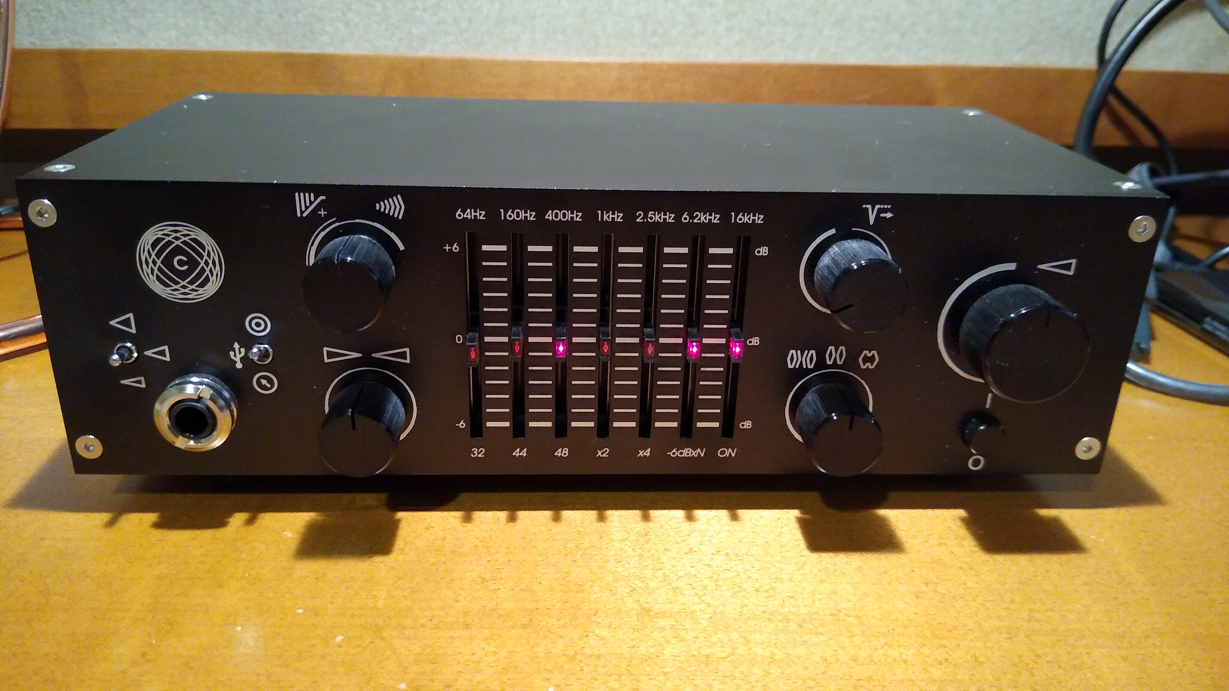
As auditioned, tested, measured

Features

I’ll review the features in the order in which I might use them most myself. With some of the features, like crossfeed and reverb, I couldn’t imagine a way to measure them. However, I did use and listen to all the features, and found that each does what it says and the effect is easily audible.

Measurements

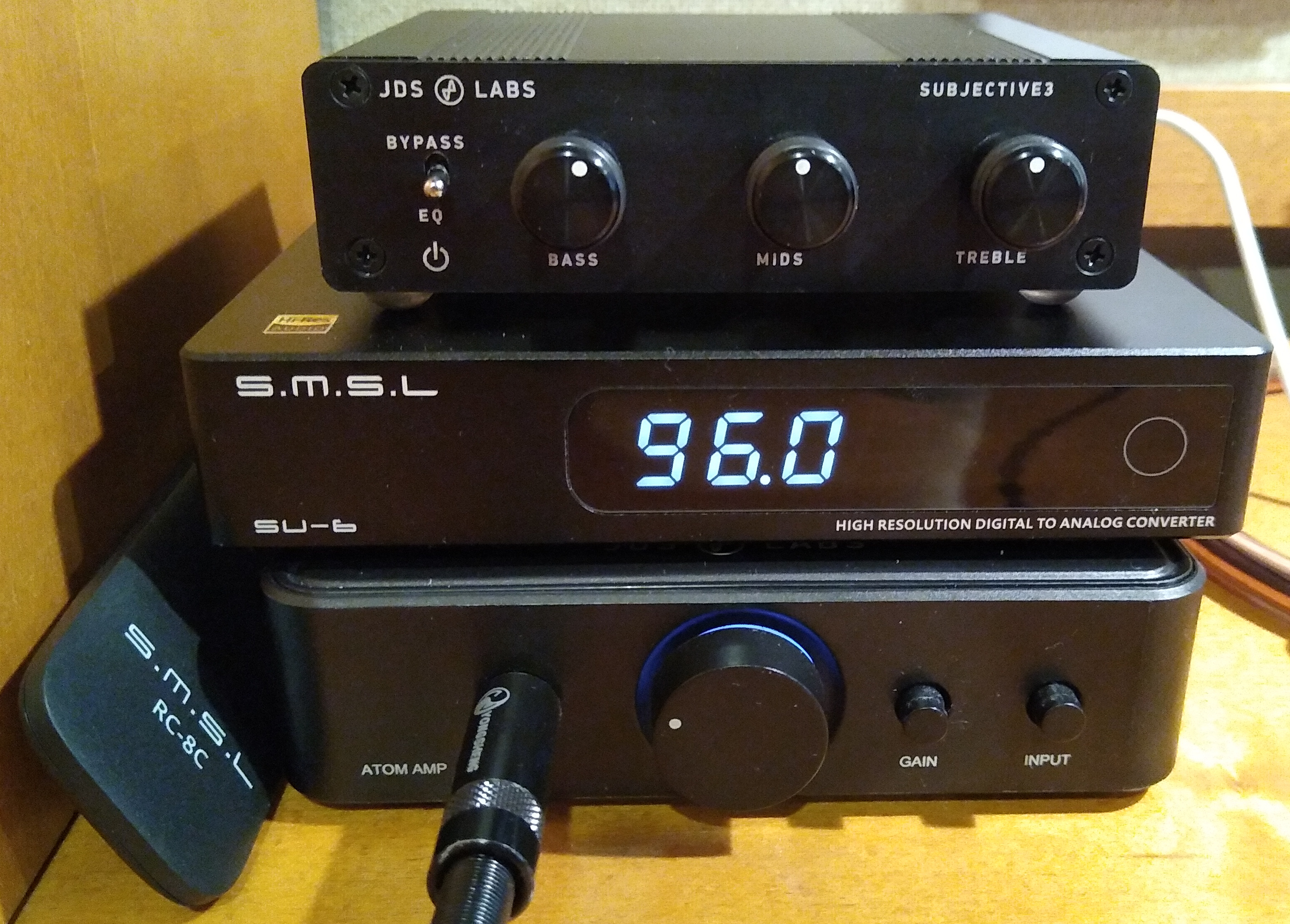
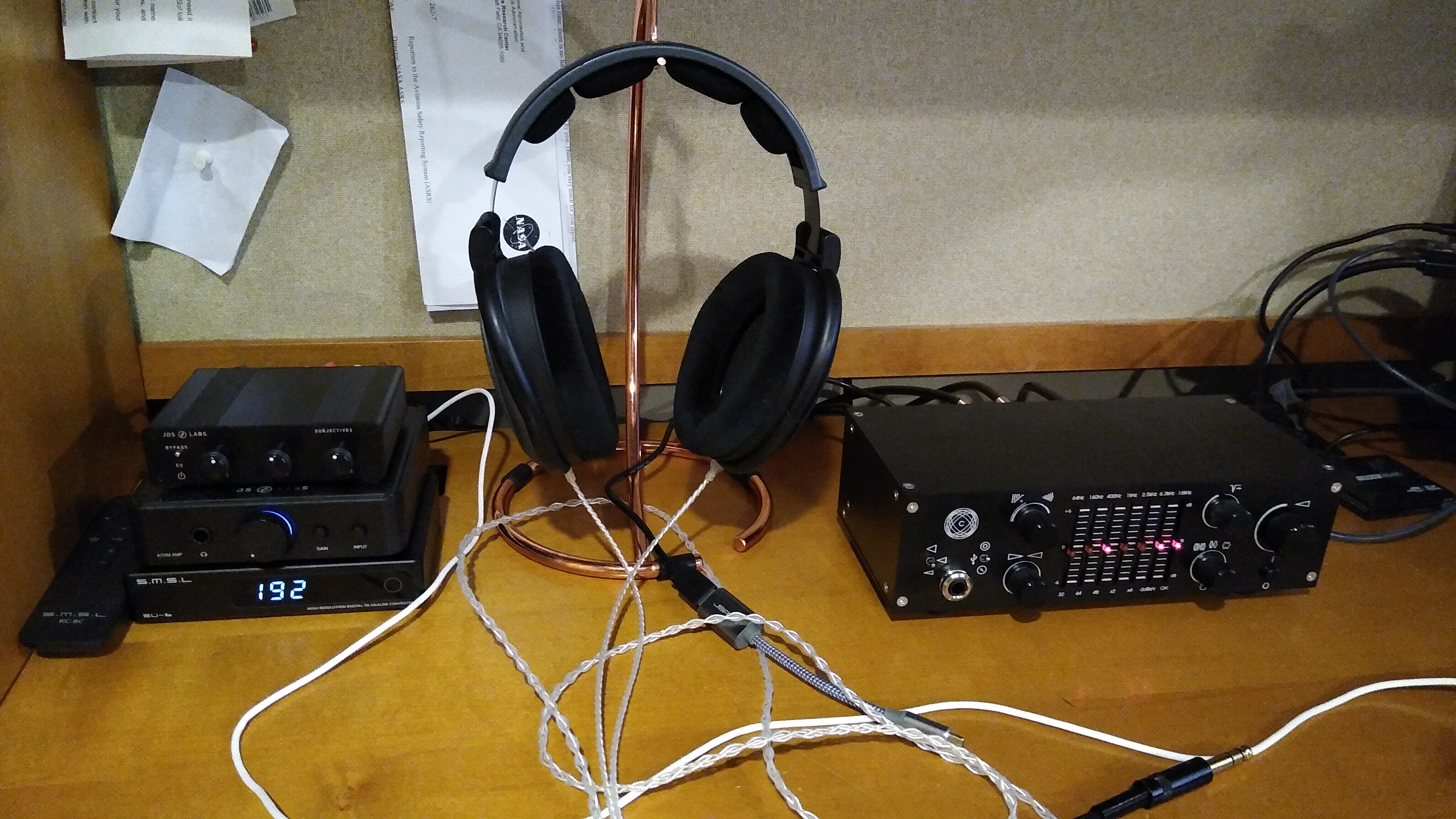
I measured the COUNTry using a PC running Ubuntu 18, an ESI Juli@ sound card, with Room EQ Wizard software. I also have an SMSL SU-6 DAC and a JDS Atom amp. The Juli@ SPDIF coax output went directly to the COUNTry. I measured it in 2 ways:

  • COUNTry analog line level outputs to Juli@ analog inputs
  • COUNTry digital SPDIF coax output to SMSL SU-6 DAC, to Juli@ analog inputs

This measured the COUNTry as an all-in-one device with D/A conversion and analog output, and also as a DSP-only device upstream from a separate DAC.

The Juli@ sound card is high quality, but it’s nothing like professional measurement equipment from manufacturers like Audio Precision. I can measure the basics (frequency response and distortion), but take the measurements that follow as directional guidance within the limitations of my equipment.

Equalizer

The equalizer’s 7 bands have equal octave spacing with frequency ratio of 2.5:1 or 1.32 octaves. They are symmetric and complementary, so they can be combined without ripple. A picture’s worth 1000 words, so here are frequency response graphs of the positive and negative ranges respectively, showing each control individually, and all combinations.

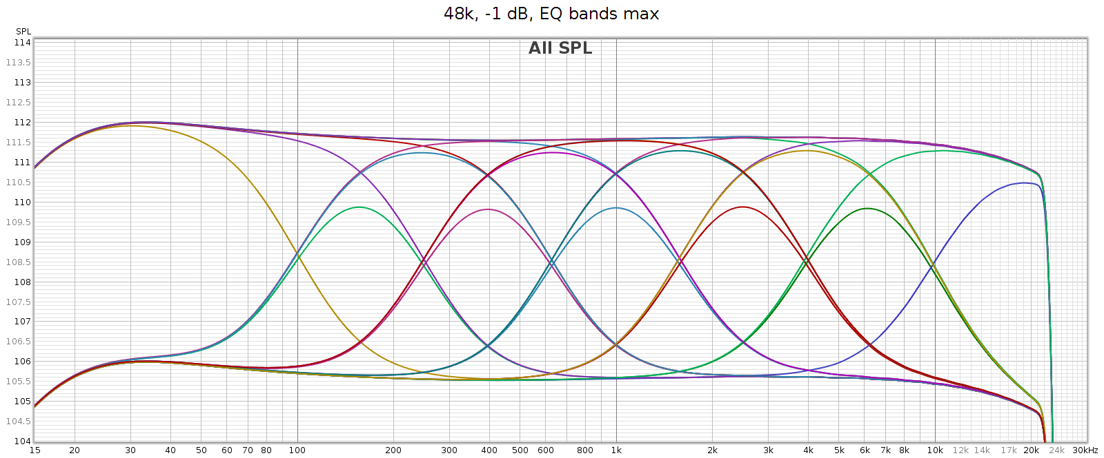
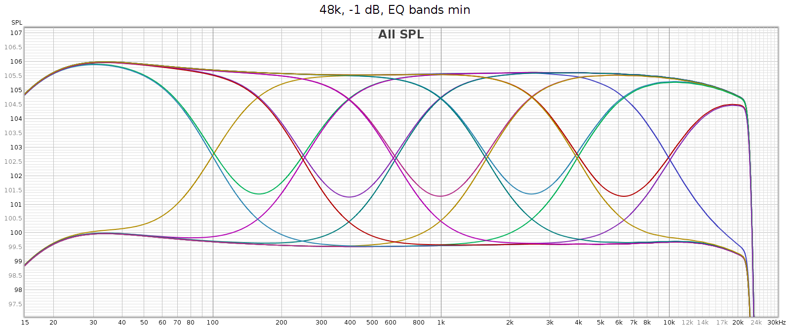
The manual says each band is +/- 6 dB, which is roughly true yet oversimplified. The max effect of any single band is +/- 4.3 dB. Two adjacent bands maxed together is +/- 5.7 dB. Three or more is 6.0 dB.

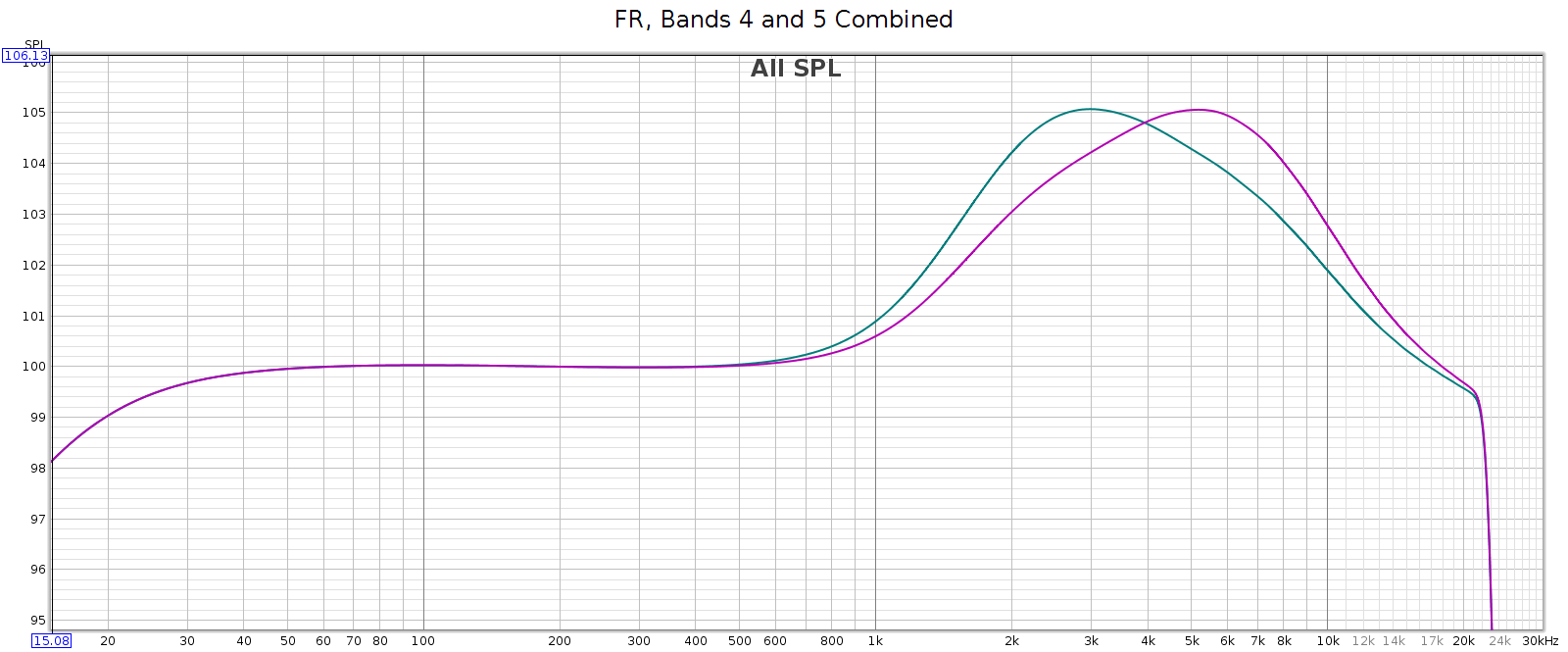
This enables adjacent sliders to be combined to form new bands. For example, consider sliders 5 and 6, centered at 2.5 and 6.2 kHz respectively. What I need to adjust the LCD-2F headphones is a slightly wider band centered at 4 kHz. And that’s exactly what I get when using both together, as you can see in the above frequency response graph. And, you can use different levels of these 2 sliders to shift the combined center frequency a bit higher or lower, to get a center frequency anywhere between 2.5 and 6.2 kHz. This makes the COUNTry’s EQ even more versatile than it appears.

For example, the following chart shows two combos: band 4 at max with band 5 at half (in teal), and band 4 at half with band 5 at max (in magenta). You can see the center frequencies are 3 kHz and 5 kHz respectively.

Regarding slider sensitivity: the following shows the center 1 kHz band at positions 1/4, 1/2, 1, 2, 3, 4, 5 and 6:

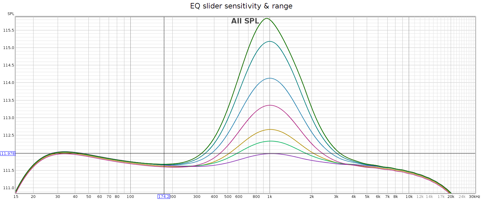
The slider effects are nearly continuous down to a fraction of a dB, allowing very small gradations. Each slider has 6 marked notches on each side (positive & negative), though only the center position is a tactile notch. The first 4 marks are about 1 dB each. The 5th mark is another 0.7 dB, and the 6th / last / max mark is the same as the 5th.

I like this design: it works like a conventional equalizer, but is more flexible. It’s a creative solution to an old problem.

Bass Boost

What: a gentle bass lift starting at 200 Hz and gradually increasing to + 6 dB at 20 Hz. This closely follows the bass attenuation of the popular Sennheiser HD-580 and HD-600 headphones, which is nice. It also mirrors the COUNTry’s bass attenuation in high gain mode, so use it if you want flat response in high gain. Its measured curve is shown twice in the following graph:

  • The top red line versus the green line.
  • The purple line versus the bottom orange line.

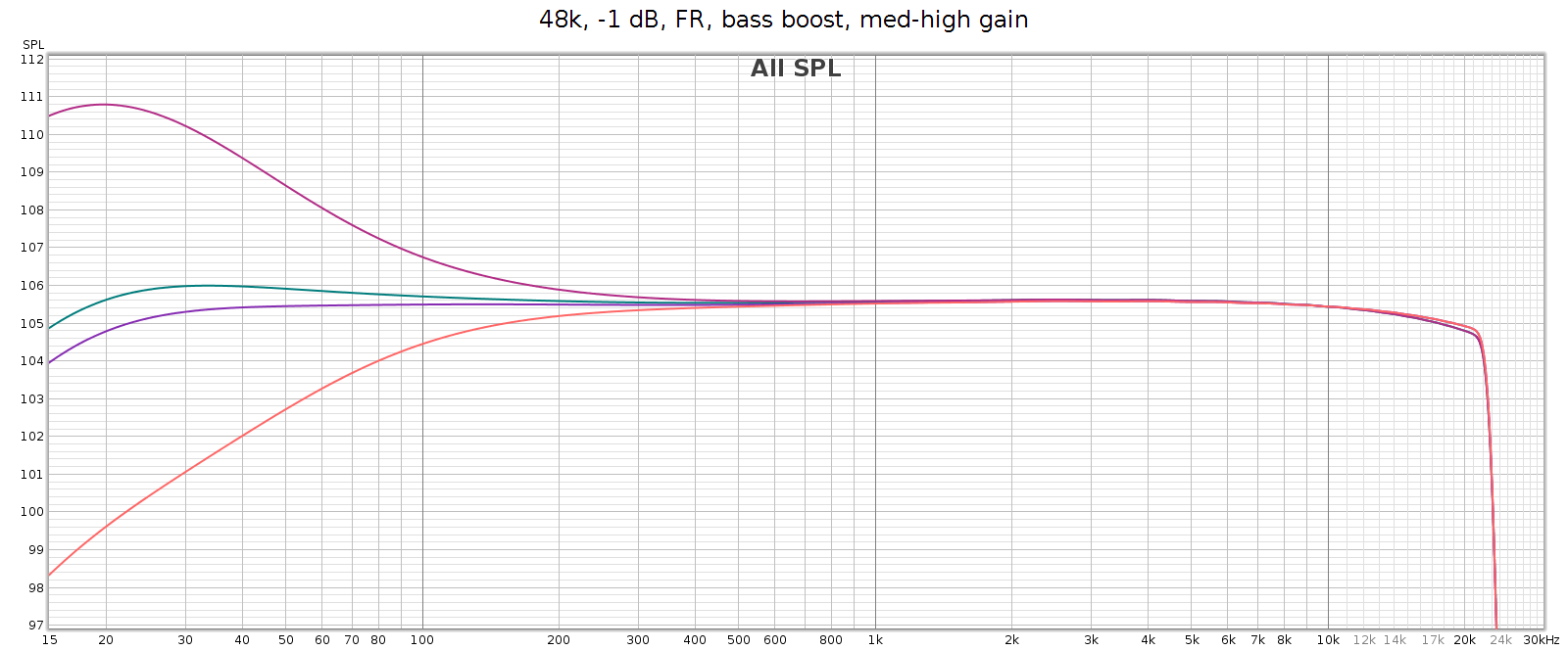
The manual says it’s a shelf boost with center frequency of 45 Hz and Q=0.5, which is true to the measured response. Q=0.5 is such a gentle slope that it is +1 dB as high as 120 Hz (evident in the above graph).

Stereo Crossfeed / Expander

Some recordings have sounds hard-panned to the left or right channels. This sounds wonky on headphones. Unfortunately, this was a common recording technique in jazz albums from the 1950s and 1960s – for example the classic Miles Davis / Coltrane album Kind of Blue. Crossfeed mixes a little of these sounds into the opposite channel, with a brief delay; it narrows the stereo separation. When listening to albums like this, it makes it sound more natural. The COUNTry has 7 levels of crossfeed (the Soul has only 5), and an 8th switch position that is mono (standard mono without crossfeed or delay). I don’t use crossfeed for normal listening, but it’s one of my favorite features because it’s so nice for those albums that need it.

Note: when clicking into mono, the sound suddenly becomes more dull. This effect is purely perceptual – the measured frequency response is exactly the same as in normal stereo.

Stereo expander does the opposite, making stereo wider. It’s intended for speakers but you can hear the effect somewhat on headphones.

Notch Filter

Many headphones have a resonance that causes a spike in frequency response in the 6k to 11k range. The COUNTry has a notch filter that cancels these spikes. Here’s the measured response of all 15 of the settings. It measures true to the specified Q=2.0, -6 dB.

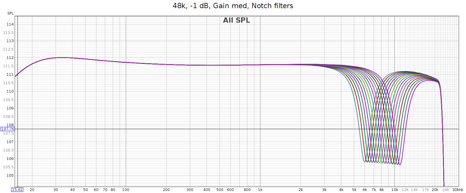
My Sennheiser HD-580 and Audeze LCD-2F don’t have such a spike, so I don’t use this feature. But the Sennheiser HD-800 does, as do many other popular headphones, making this a useful feature.

Reverb

This does exactly what it says: it adds reverb to the music. I’ve tried it with various recordings across a variety of musical styles from classical, to jazz, rock, etc. It’s not my cup of tea, as I prefer dry recordings. Yet this is a personal subjective thing. The reverb sounds natural and well implemented, and has 3 levels to play with.

Volume Control

The volume control feels analog but is digital, having perfect channel balance at every step from max to min. It also lights up an LED at certain exact positions: 0 (max), -6, -12, -18, and -24. This is useful for setting levels to avoid clipping when using DSP features.

Analog Gain

The COUNTry has 3 gain levels for its analog outputs: low, medium and high. Strangely, in high gain it attenuates low frequencies. The manual says this is to reduce excessive excursions of drivers at high levels. This doesn’t make sense to me, since high gain would be used for low sensitivity headphones or amps that need more voltage for the same sound level. And the COUNTry enables you to adjust the low frequencies if you want to. However, the bass boost switch exactly mirrors this bass attenuation, so if you are using high gain mode, turn on bass boost to get flat frequency response.

We’ve heard the mantra “the more gain, the more pain”. This is generally true, due to the constant gain * bandwidth of the transistors & opamps used in amplifiers. Because of this, the best approach is normally to use low gain whenever possible. That is, for a given loudness level, low gain at a higher volume position is usually cleaner than medium or high gain at a lower volume position. This also preserves digital resolution.

Note: This is especially true with conventional analog potentiometer volume knobs, which typically have better channel balance at high settings. However, the COUNTry's digital volume control has perfect balance at all settings. So that's not a factor here.

To test how the gain affects noise & distortion, I measured the COUNTry noise & distortion at each gain setting, with volume adjusted so that each had the same output level. Because the volume knob is digital, I couldn’t match the levels exactly, but I could match within 0.3 dB. More specifically:

  • Low gain at volume -6 dB
  • Medium gain at volume -16 dB
  • High gain at volume -26 dB

Medium gain measured slightly cleaner than high gain, but only slightly. Low gain was about the same as medium gain. So with the COUNTry, the gain level you use doesn’t make a significant difference in distortion or noise. Just select the gain that matches the sensitivity of the downstream device the COUNTry is driving. Of course, remember that high gain attenuates bass so use the bass boost to get flat response.

CD De-Emphasis

As mentioned above, the 7 band EQ has a creative design that eliminates ripple across the bands and enables adjacent bands to be combined to shift center frequencies. However, the highest band (16 kHz) has a special feature. When set to the minimum, it applies the Redbook CD de-emphasis curve. It’s nice to be able to apply this manually since some old CDs use it, they sound much too bright unless it’s applied, and many aren’t formatted properly for DACs to recognize and apply it automatically.

However, the equalizer slider has no indication when this triggers. It triggers at the bottom position, but as you raise the slider, it moves a short distance before disabling de-emphasis and attenuating the 16 kHz band. If you want the most 16 kHz attenuation without triggering de-emphasis, you must do it by ear. Slide it all the way to the bottom, then slowly lift it until the sound suddenly gets a bit brighter. It would be nice to have an indicator that lights up when de-emphasis is activated. The LED on the 16 kHz hand is already used as a power indicator, but it could be made to blink when de-emphasis is activated.

Miscellaneous

The measured impulse response is symmetric and phase response is flat into the high frequencies, which means the COUNTry uses standard linear phase filtering, rather than minimum phase.

The case and knobs are constructed in a manner that appears easy to disassemble and service. It’s good to see this exception to our modern age of cheap disposable equipment. I did not test this by opening the unit, since it is just a loaner.

Support is excellent. You can contact Jan Meier of Meier Audio directly on the company website or on Head-Fi. He is responsive, knowledgeable and helpful.

Usage and Build Quality

The COUNTry is a nice little device with an unusual look. It’s an “old-school” look and feel with physical knobs and LEDs instead of a display screen with menus. It has high build and parts quality.

Some of the indicators are a bit obscure but they become intuitive as you use them. For example, the digital sample rate display is done with 2 LEDs. One for the base rate (32, 44, 48) and another to indicate a multiplier (2x or 4x). Another LED lights up when the volume control is exactly at certain positions: 0 (max), -6 dB, -12 dB, -18 dB and -24 dB. This is a nice guide for setting precise levels.

The rotary switches make a solid “snap” and feel like professional test gear. The toggle switches are similar. The EQ sliders feel like potentiometers,  smooth with just the right amount of friction. The COUNTry is fully digital, so it detects the slider position and translates to a digital value. There is a tactile detent for the center position, but no others indicating when it’s shifted from one value to another. The controls feel good to use.

The headphone jack is seriously robust and overbuilt. The back panel connectors are not as robust but still feel solid. This makes sense as the headphone jack is likely to be plugged & unplugged much more often than the rear connectors.

Sound Quality (Subjective)

OK so what does it actually sound like? I listened on my Sennheiser HD-580 headphones. They are over 20 years old, but have fresh pads and I recently tested them with a MiniDSP EARS rig. They still have measured performance like new. I also used Audeze LCD-2F headphones (also tested & measured). The sound source was my PC with its ESI Juli@ sound card, and lossless FLAC files at bit rates ranging from 44.1 to 192. The Juli@ card coax SPDIF output routed to the COUNTry. I routed the COUNTry’s SPDIF digital output to my SMSL SU-6 DAC and JDS Atom headphone amp. With this setup, I could plug the headphones directly into the COUNTry, or into the JDS Atom. This enabled me to test the differences (if any) between the COUNTry in pure digital mode, versus its D/A and analog outputs.

I level matched by playing white noise, routing the analog outputs to my Juli@ card and measuring the level. With the JDS Atom’s analog volume knob, this enables level matching to about 0.1 dB.

In a word, the COUNTry sounds just a bit brighter than the SU-6 + JDS Atom. I first noticed this with music, and confirmed it with pink noise, which is a useful test signal for hearing subtle differences in frequency response. This brightness was unexpected, since the COUNTry’s analog frequency response has a slight bass boost and treble cut. However, the brightness sounds like it’s in the upper mids / lower treble, rather than in the highest frequencies. Loud parts with many instruments playing (like a symphonic crescendo) are slightly less resolved on the COUNTry analog output, compared to the SU-6 + JDS Atom.

Subjectively, the COUNTry analog output has a good clean sound across a variety of music with no obvious issues or artifacts. Though it’s not state of the art in terms of linearity, smoothness or detail – nor was it intended to be. Think of the COUNTry analog outputs as a sonically competent add-on feature. The COUNTry digital outputs are more transparent.

When you plug in headphones while the COUNTry is playing, it sometimes emits two loud CLICKs in the headphones, then pauses for about 1 second before the music starts. Inserting the headphone plug quickly usually avoids this. Meanwhile, the line level outputs are always playing and do not pause or CLICK. If you power on the COUNTry while it has musical input, you get a single loud CLICK then the sound starts playing in the headphones.

Anomalies

Frequency Response

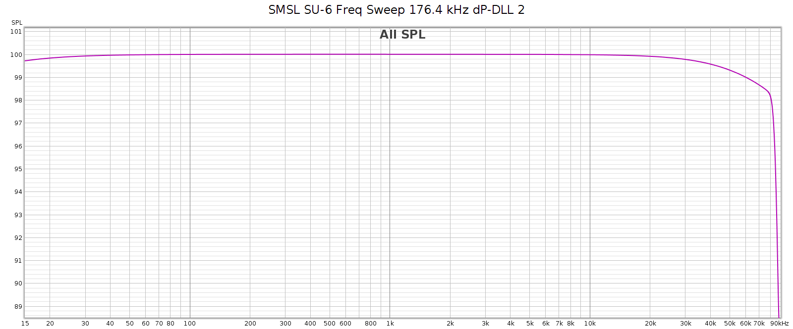
Analog frequency response is not quite flat, and different in low (blue), medium (green) and high (red) gain. Medium gain has a 0.5 dB lift in low bass, and high gain has a 6 dB drop in low bass. All modes gently taper high frequencies, reaching about -0.6 dB at 20 kHz.

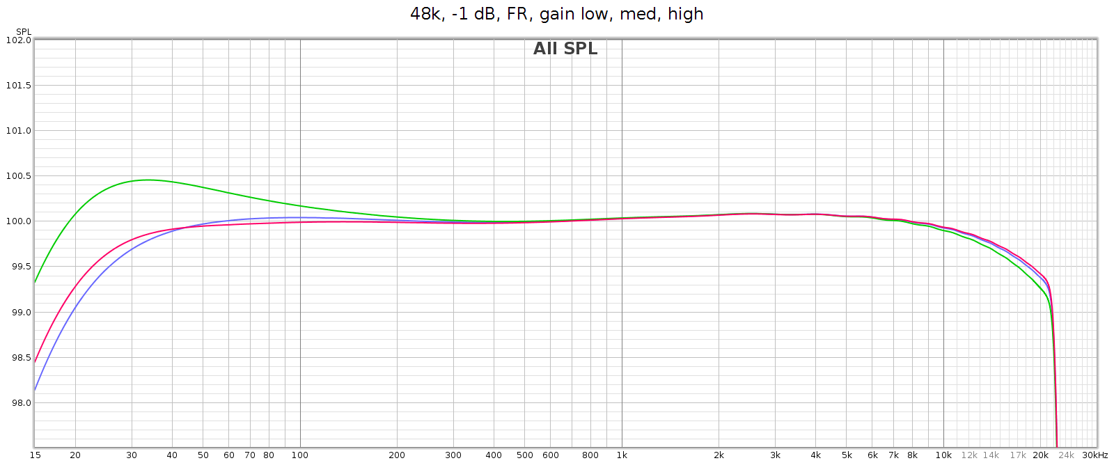
Note: in the above high gain curve (red), digital bass boost was applied to flatten the response. The uncorrected response is shown in another graph below.

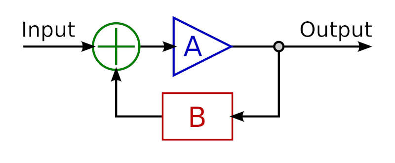
Why the frequency response differences at different analog gain levels? This is due to the Meier Audio FF or Frequency Adaptive Feedback. It attenuates low frequencies in the digital inputs, then boosts them back to flat again in the analog outputs. This means the attenuation curve (implemented in DSP) must match the boost curve (implemented in passive analog components). Meier Audio optimized this matching at low gain, since they expect that will be most often used. The purpose of FF is to frequency shape and optimize DA conversion and the gain-feedback loop, so it is only used for the analog outputs, not on the digital outputs.

As mentioned above, in high gain the frequency response attenuates bass beginning at 200 Hz, gradually reaching -6 dB at 20 Hz (this is noted in the manual). The COUNTry has a DSP bass boost that applies the exact reverse of this. So if you want flat response in high gain mode, turn that on (as it is in the above graph).

Let’s take another look at the bass boost frequency response graph shown earlier. From bottom to top:

  • Orange is high gain
  • Purple is high gain with bass boost activated
  • Green is medium gain
  • Red is medium gain with bass boost activated

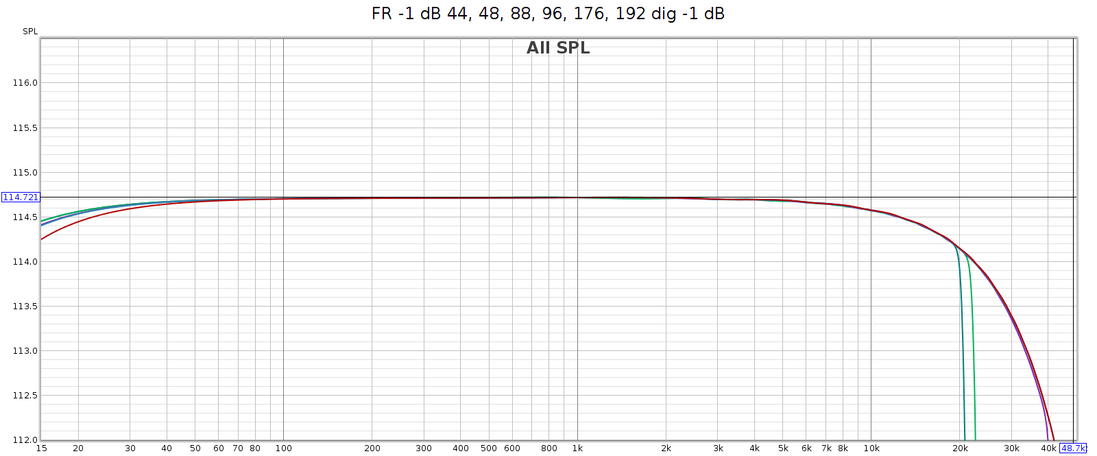
The COUNTry’s digital output is smoother and more linear, but still has gentle HF attenuation reaching -0.6 dB at 20 kHz, and even gentler LF attenuation about -0.2 dB at 20 Hz. We see below that this slight attenuation happens in the digital domain. This graph shows the digital output with all sampling rates on top of each other:

Noise at High Sample Rates

At high sample rates (176.4 and 192) the COUNTry has a lot of high frequency noise. This is unexpected and unusual, so I tested in several different ways:

  • Analog outputs
  • Analog outputs at lower levels (-6 dB, -12 dB)
  • Analog outputs with lower digital input levels (to -48 dB)
  • Analog outputs with input from my phone (USB Audio Player Pro) in bit perfect mode, instead of from my computer (ESI Juli@ sound card)
  • Digital outputs
  • Digital outputs at lower levels (to -48 dB)

It measured the same in all cases. This suggests the issue is not in the D/A conversion or analog stage, but in the DSP.

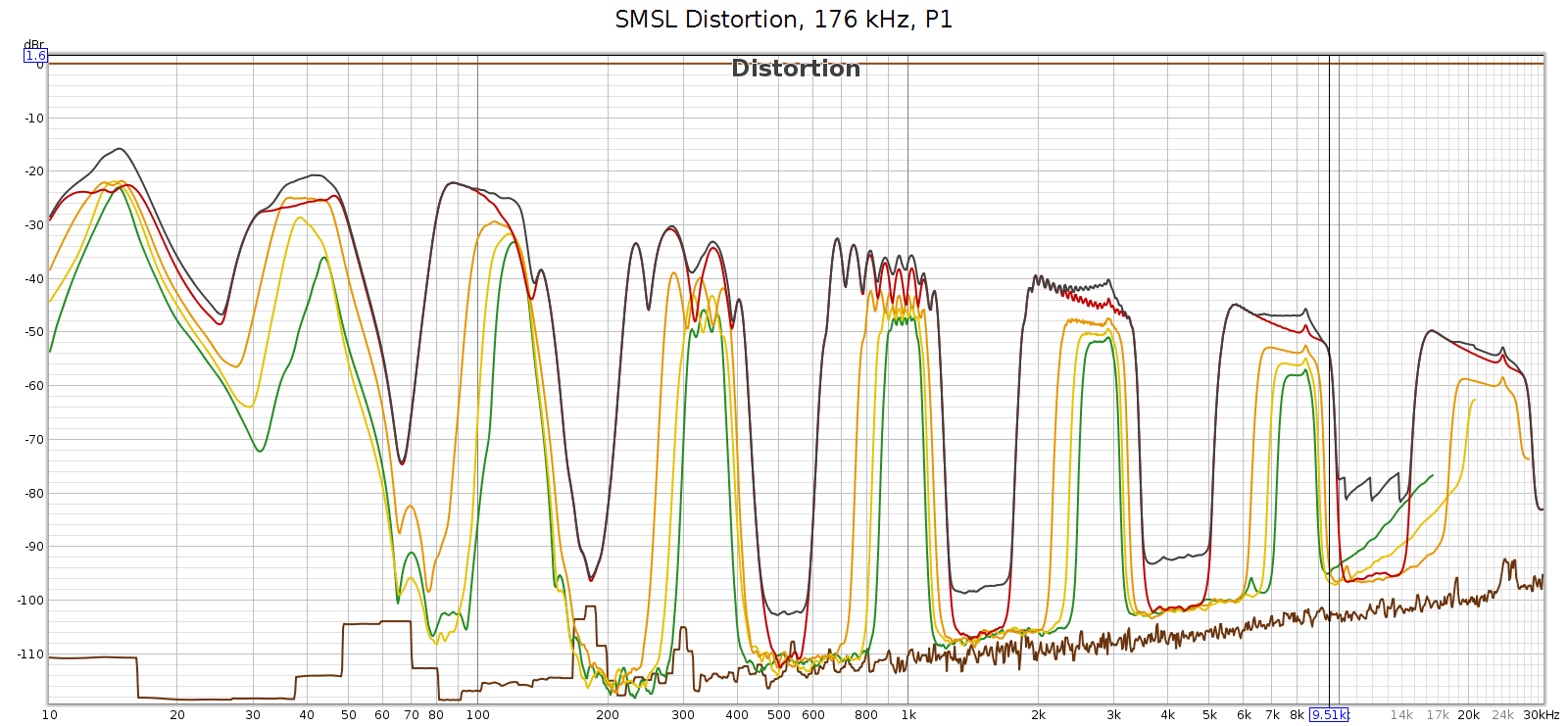
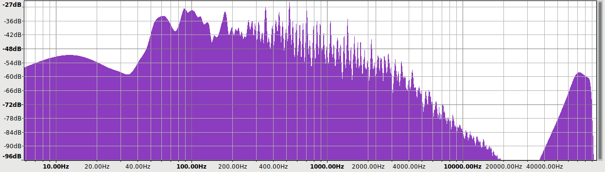
Here’s what that noise looks like at 176.4 kHz. Actually, in the graphs below it looks like distortion rather than noise, but more on that later. The horizontal line at y=0 dB is the sweep signal. It is not really at 0 dB, but this is relative to facilitate reading the levels. The brown line is noise. The black line is THD. The colored lines are 2H, 3H, etc., which sum to the black line.

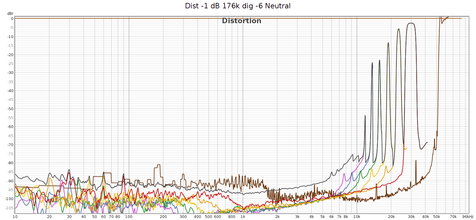
At 176.4k, it’s clean up to 11 kHz and that first distortion spike is at 11,960 Hz. This is inaudible since it’s 7th harmonic so the distortion tone is at 11,960 * 7 = 83,720 Hz. However, these distortion spikes are big enough that their intermodulation (IM) differences are in the midrange. They are spaced 1-3 kHz apart, which puts the IM smack-dab where our hearing is most sensitive to it.

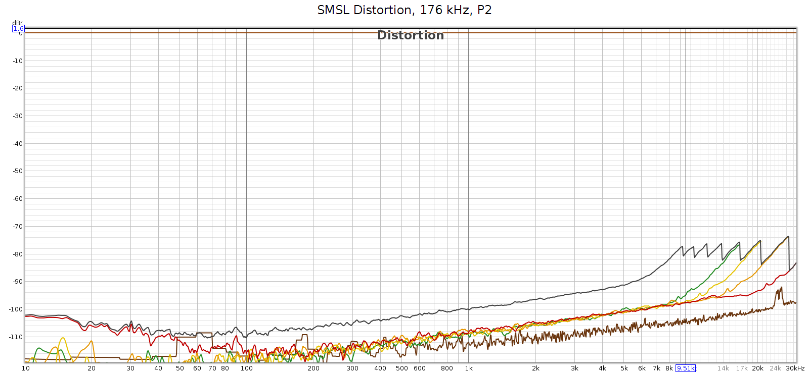
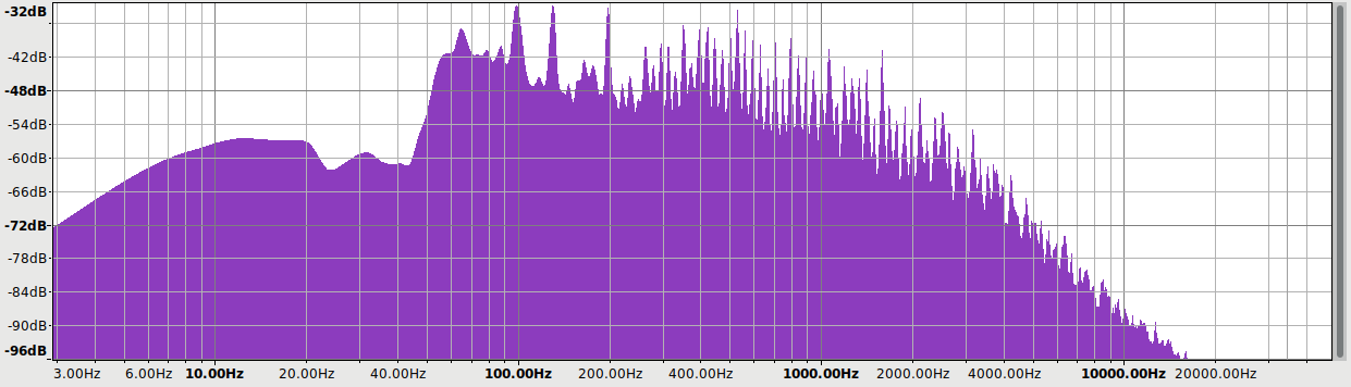
Here’s what it looks like at 192 kHz:

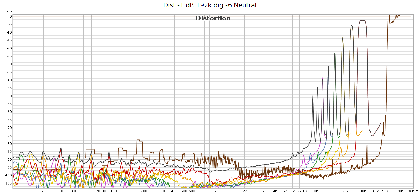
At 192k we have a similar situation, first distortion spike at 9,580 Hz, which will be inaudible since it’s 9th harmonic so the distortion tone is at 9,580 * 9 = 86,220 Hz. The 7th, 6th, and rest of harmonics are the same as at 176.4k sampling. And as above, the IM difference tones will be in the midrange.

Two interesting observations about these frequencies:

  1. They are exactly the same at 176.4 and 192 kHz. This suggests it is noise, not distortion – it’s not correlated with the signal.
  2. They all point to noise in the same region: 53 to 86 kHz

More precisely:

  • H9 @ 9,580 Hz means a frequency at 86,220 Hz
  • H8 @ 10,620 means 84,960
  • H7 @ 11,960 means 83,720
  • H6 @ 13,640 means 81,840
  • H5 @ 15,870 means 79,350
  • H4 @ 18,940 means 75,760
  • H3 @ 23,320 means 69,960
  • H2 @ 30,000 means 60,000

Here’s my speculation as to the root cause. Something in the COUNTry (perhaps a switching power supply?) is operating at 65 kHz. This is not fully suppressed or filtered and is leaking (somehow?) into the digital data. At sample rates 96k and lower, it’s above Nyquist and thus digitally filtered. But at 176.4 and 192, it’s below the Nyquist limit of 88.2 and 96 kHz respectively, so it is in the passband. Thus this power supply switching noise appears as harmonics of the given lower frequencies. If so, then it’s not really distortion, it’s noise.

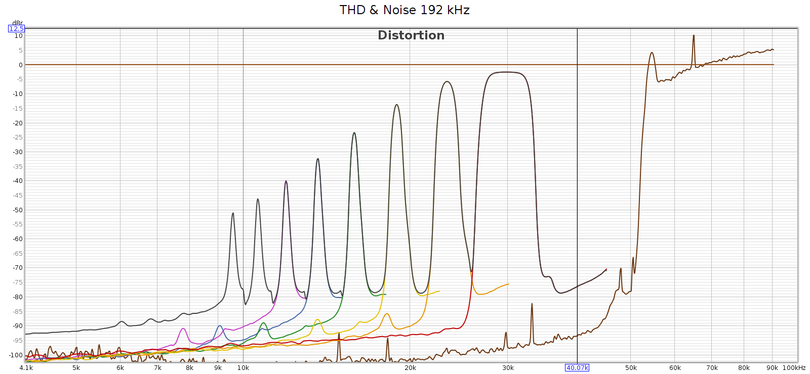
Wherever the source of this noise, it’s interesting to study it closer. I created another graph below for this. Noise goes through the roof (literally – greater than 100% or louder than the fundamental) with spikes at 54.6 and 65 kHz. This noise profile and the spike frequencies are exactly the same at 176.4 and 192 kHz, so it’s independent of sampling frequency. It looks like this noise is what the graph (incorrectly) shows as distortion. Each of the N harmonic spikes is simply that same noise frequency divided by the next larger number (2nd, 3rd, 4th, etc.). Note that noise above the 0 dB line is not a bug. The spike at 65 kHz at +10 dB means it’s 10 dB louder than the signal.

In case this noise were caused by the high level of the digital signal (even though it wasn’t clipping), I ran another sweep at -48 dB. The noise profile looks the same:

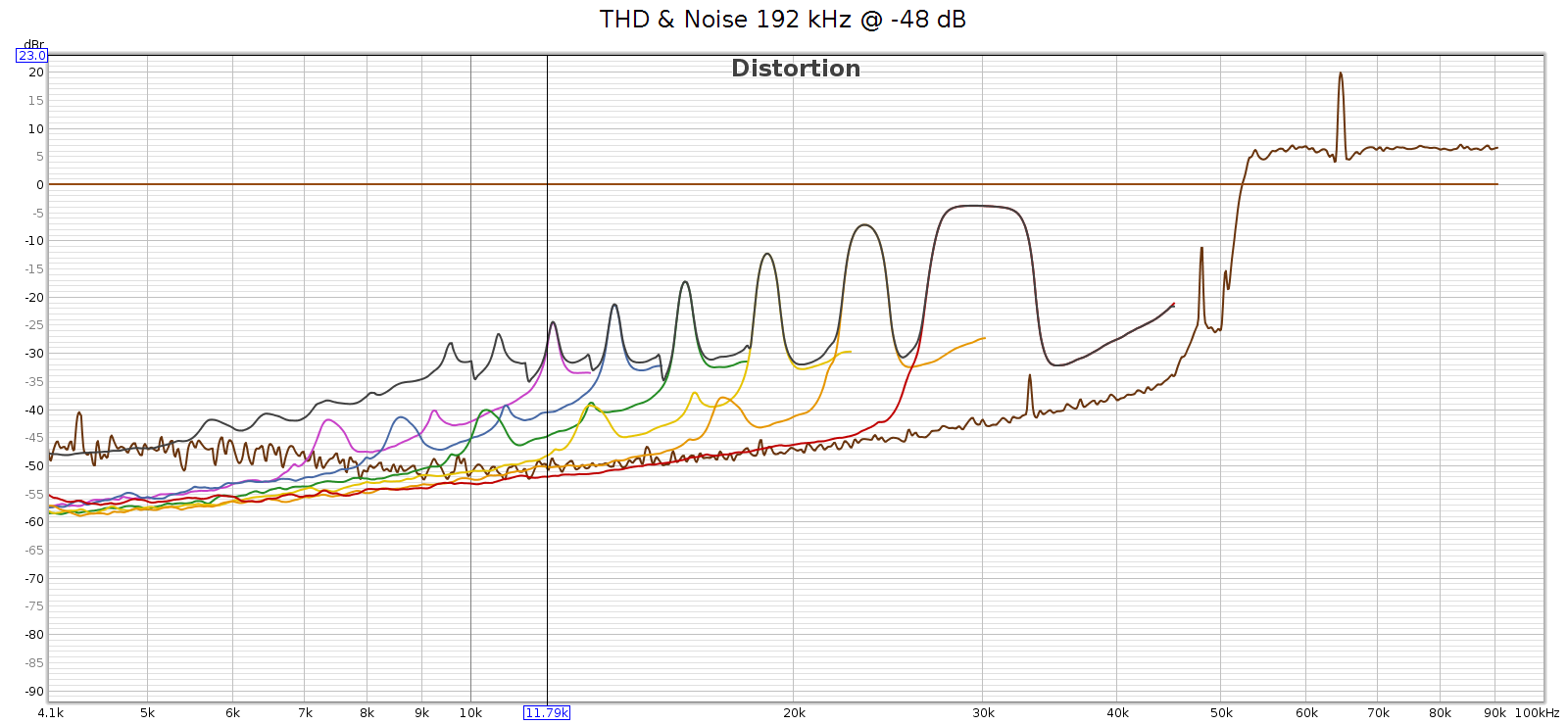
In short, the noise is a constant level, and a constant frequency spectrum. It’s independent of the sample rate and of the input signal. This suggests it’s noise not distortion.

I said earlier that I was speculating – let me clarify. What is not speculation, but observation, is a lot of supersonic noise at high sample rates. My speculation is toward the root cause. I love a good puzzle and this explanation fits the observations. But I don’t really know what is causing that noise. So let’s set root cause speculation aside…

For comparison, here’s the COUNTry distortion and noise at 96 kHz, measured at the analog outputs at medium gain:

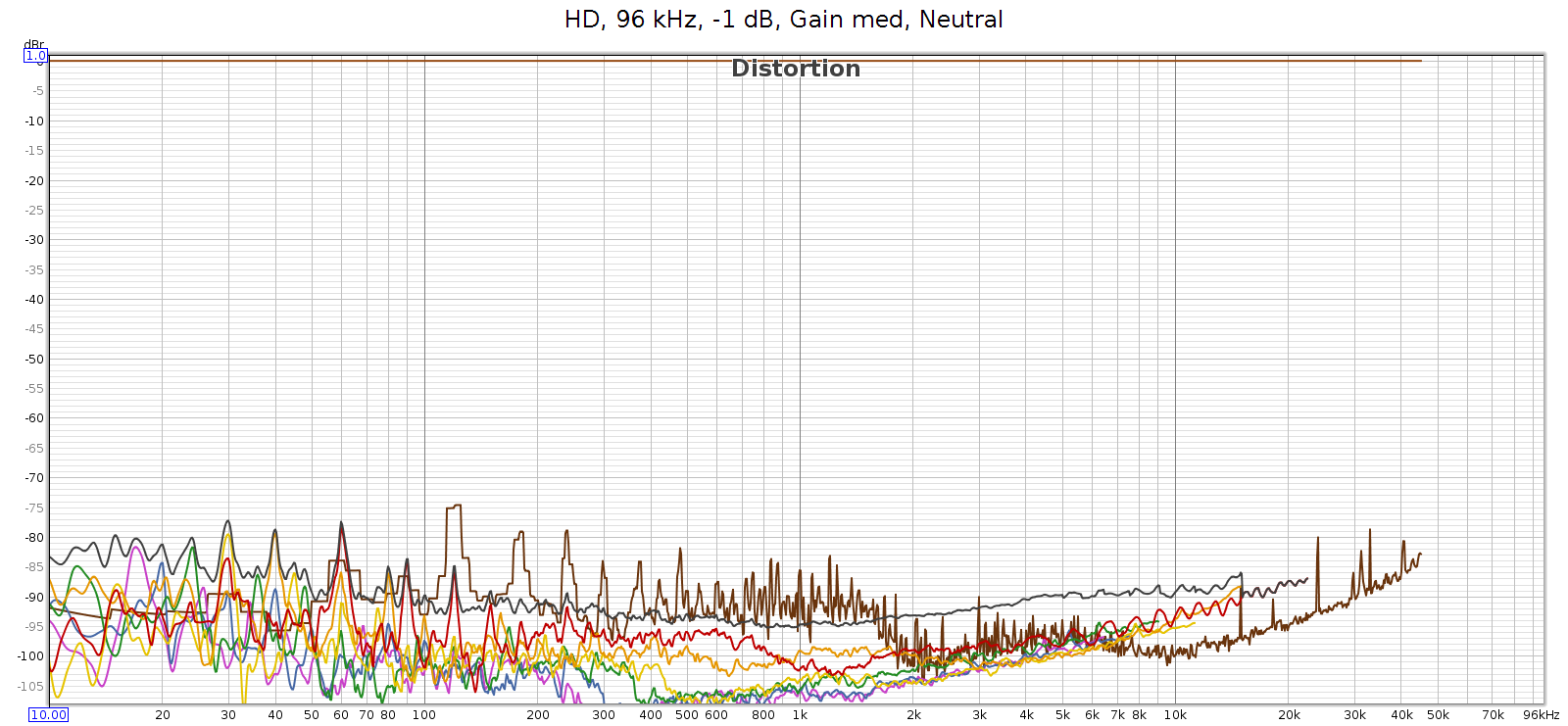
BTW, see that drop in noise & distortion from 700 to 2,000 Hz? I’m guessing this is the previously mentioned FF at work.

Here’s the distortion and noise of the measuring system, my ESI Juli@ sound card in loopback:

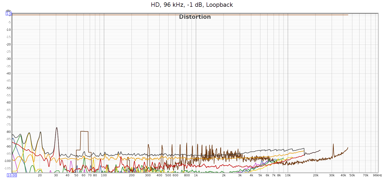
This typical of all sample rates 96 kHz and lower. So the COUNTry’s D/A and analog output is pretty clean – just a bit higher than the loopback connector, but not much. This should be well below audible levels.

Finally, I used Audacity to under-sample the 192 kHz test signal to 96 kHz, then played it through the COUNTry. The output looked clean, just like the 96k signal above. As expected.

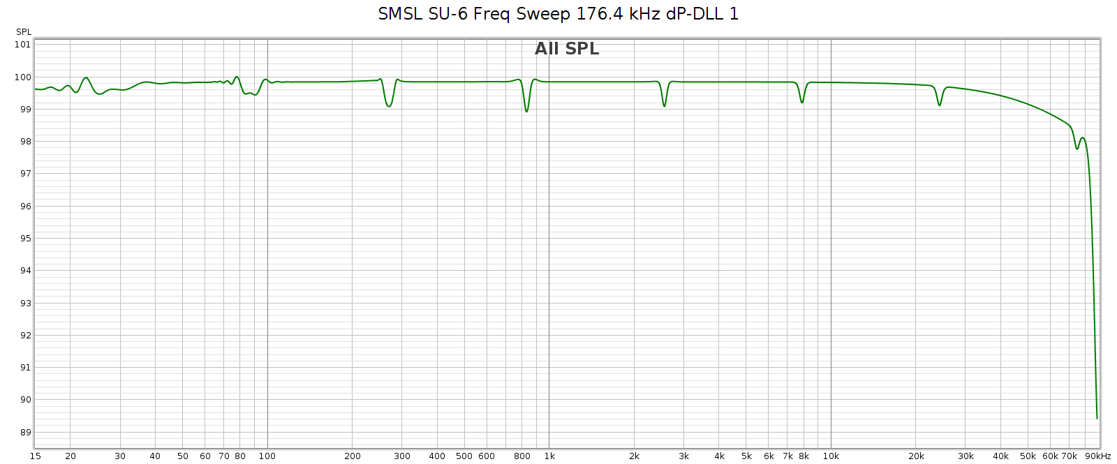
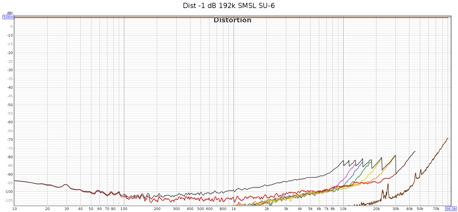
Just in case the issue was with the 192 kHz tone itself, I measured how the SMSL SU-6 reproduces that test sweep signal, directly without the COUNTry. You can see those rising harmonics, but they cut off around -80 dB. This is the inherent noise and distortion of the Juli@ card’s analog input and A/D converter.

Conclusion

The COUNTry is a unique device. At 1 kilobuck it’s rather pricey, but considering its functionality, as an all-in-one device it replaces several others: DAC, amp and EQ with DSP. If you bought these separately, the total cost might be similar. And the COUNTry’s DSP features are unique and well implemented – you might not be able to find such a flexible EQ, or DSP with crossfeed or reverb. It’s built to last and the sound quality, both measured and subjective, is quite good if not state of the art. Used in purely digital mode, it should be sonically transparent, at least up to 96 kHz.

Meier Audio sent me one on request because I was curious about it. I don’t get to keep it. Yet over an extended trial using it nearly every day, here’s what I like best about it:

  • The flexibility of the EQ (shifting center freqs by combining adjacent bands) enables me to match the LCD-2F and HD-580 headphones, and most others.
  • The crossfeed is nice especially with albums having hard-panned L-R stereo separation.
  • Flexibility to be an all-in-one device or run in digital-only mode.
  • Works with my various audio systems with no observed software/firmware bugs.
  • Good quality, seems built to last with good support.

Suggestions for improving the COUNTry:

  • Fix the HF noise/distortion issue at high sampling rates.
  • For improved transparency, make a version that run DSP at the native sampling rate of the source without resampling.
  • If native rate processing is not possible, then over or under sample at integer multiples. Example:
    • Implement all internal functionality at 2 rates: 88.2 & 96
    • Input at 44.1, 88.2 and 176.4 process at 88.2
    • Input at 48, 96 and 192 process at 96
  • Provide an indicator when CD de-emphasis is activated (perhaps make the 16k EQ band light blue instead of read, or blink).
  • Eliminate the bass attenuation in high gain mode.
    • Sure you can normalize it with bass boost, but better to give it flat response like low & medium gain.
    • Not really an issue for me, since low gain is plenty for my headphones.
  • One of the nice things about the COUNTry is that due to the physical knobs you can see all the modes at a glance. But the knob detents are hard to see. If I owned this device I’d fill the detent notches with white paint.

Of the above, the the only thing holding me back from buying one for myself is the first 2 items. Eliminating the high frequency noise and not resampling might also improve the clarity / transparency / sound quality.

Meier Audio makes another version of the COUNTry that resamples everything to 96 kHz instead of 192 kHz. This 96k version has a more complex implementation of bass boost, called bass enhancement. It’s quite an interesting feature that leverages the psychoacoustic phenomena known as the “false fundamental”. As cool as that is, this 192k version has certain advantages, even if one doesn’t care about the difference in sample rate:

  • Bass boost exactly offsets the analog bass attenuation at high gain. The 96k version has no way to do this, since it replaces boost with enhancement.
  • Bass boost closely offsets the bass attenuation of several headphones, especially the Sennheiser HD 580/600/650/800 models.

Note that neither of the above reasons has anything to do with 96k versus 192k sample rates. In my opinion, 192k offers no real advantage over 96k because whatever advantages are gained from rates higher than the 44.1k CD standard, are fully realized at 96k.

Update: Apr 2023

Meier audio has a new version of the COUNTry:

  • Performs all DSP at the native sample rate (32, 44.1, 48, 64, 88.2, 96, 128, 176.4, 192)
    • Digital-only mode has no resampling, should be fully transparent
  • D/A conversion is always done at 96k, since the WM8716 chip is optimized for this rate
    • The analog audio output is resampled to 96k before D/A conversion
  • Equalizer step sizes are 0.5 dB resolution
  • Reverb replaced with 3 levels of bass boost (50 Hz shelf, Q=1.0) +2, +4 and +6
  • The original bass boost (45 Hz shelf, Q=0.5, +6 dB) is retained, and can be applied in addition.

Analog vs. Digital

From Merriam Webster:

Analog

  1. of, relating to, or being a mechanism or device in which information is represented by continuously variable physical quantities
  2. something that is similar or comparable to something else either in general or in some specific detail : something that is analogous to something else

Digital

  1. composed of data in the form of especially binary digits
  2. of, relating to, or using calculation by numerical methods or by discrete units

In terms of storing, transmitting and playing audio, each term is ambiguous, yet their different meanings are similar, which leads to confusion.

Analog

The key phrase with meaning 1 is “continuously variable”. A turntable needle tracking a record groove, a tape deck head responding to fluctuating magnetic fields on tape, are both continuously variable. Reflective and non-reflective spots on a CD are not continuously variable – it either reflects a laser beamed at it, or it doesn’t. A square wave transmitted along a wire is not continuously variable – it is either at its max voltage, or its min voltage, nothing in between.

However, if we look more closely at the last two examples, we realize that they really are continuous. A reflective spot on a CD doesn’t reflect back 100% of the light; it’s not perfectly smooth, some of the light is scattered and lost. Conversely, a non-reflective spot does reflect back some tiny amount of the light, even though it absorbs or scatters most of it. And while all the spots of the same type (reflective or not) are similar, they are not exactly the same; each is unique. A square wave does not switch from high to low, or low to high, instantaneously. That would require infinite rise time, which is impossible. And as it approaches the new voltage, it will overshoot or undershoot just a bit before it stabilizes. So the voltage actually does vary continuously from the high to low value, even if it spends 99.99% of its time at a high or low value. In this sense neither of these are as discrete as they first seem; they are almost but not quite discrete, but actually continuous.

In fact, the universe at the super-macro atomic scale at which we perceive and manipulate it, is continuous. It only becomes discrete at the subatomic/quantum level.

The other sense of “analog” is that it is an “analog” of, or actually resembles the thing it represents (closely related to the word “analogy”). A magnetic tape that encodes music, has a strong field where the music is loud and a weaker field where it is quiet. A turntable needle tracking a record groove physically moves over a bigger amplitude when the music is loud, smaller when it is quiet. The shape of the groove itself resembles the waveform of the music being played.

Music as we experience it, and as it passes through air as vibrations and pressure changes, is continuously varying. Analog storage of music fulfills both definitions of the term: it is continuously varying, and it physically resembles the music (in some way, directly or indirectly).

Digital

The first definition refers to binary digits. However, this does not fully capture the sense of what it really means. The rational numbers are continuously varying, in the sense that they are infinitely dense: between any two of them, no matter how close they are, lie infinitely many more. Mathematically, the rational numbers are not a true “continuum”, as they have holes – by holes I mean numbers that we know must exist since they are the solution to simple algebra problems, yet are not rational. For example, the square root of 2.

Yet pragmatically speaking, this is a distinction without a difference. It is impossible to detect the difference between rational and real numbers through observation or measurement of the physical world. For every irrational number R, for any small value ε, we can pick a rational number Q so that | R – Q | < ε. We can pick ε smaller than any means of physical observation or measurement. Indeed, ε can be smaller than relativistic uncertainty principles permit. So even in theory, not just in practice, it is impossible to discern the difference in the physical universe. The difference between rational and real numbers does exist, but it is a mathematical distinction, not a physical one.

So for purposes of analog vs. digital, the notion of “infinitely dense” is a sufficient interpretation of what “continuous” means. Numbers can be continuous. Of course, numbers can also be non-continuous or discrete: like the counting numbers.

Even binary digits can be continuous. Every rational number can be expressed in binary digits, though some of them require infinitely many binary digits. For example, 1/7 in binary is 0.001001001… but that is still a well defined and valid number. When people use the term “binary digit” they often mean stored in a computer. But binary is simply a numbering system. It can be, but doesn’t have to be, stored in a computer.

However, in a computer the manifestation (storage, transmission, computation) of numbers is necessarily finite. Thus these numbers cannot be “infinitely dense”, which means they cannot be continuous. They are discrete numbers – even floating points, because they have finite resolution.

Because numbers can be either continuous or discrete, they are a poor concept on which to base the definition of “digital”. So much for Webster’s definition 1; that colloquial usage leads to confusion.

A better concept is definition 2: that of being “discrete units”. Storing or encoding data as a set of discrete states. We often use computers and binary, but the number of states is immaterial: it can be 2 (binary), 3 (trinary) or whatever.

In short, a big part of the confusion around the term “digital” is this: Just because it uses numbers, doesn’t mean it must be discrete. And just because it’s discrete, doesn’t mean it must use numbers.

Digital audio is discrete, and it uses numbers. The first is essential, the second is an incidental convenience.

Once again: truly discrete phenomena do not exist in our universe at the super-macro atomic scale. Discrete means a set of states with nothing in between the states. This is easy to understand from an abstract logical perspective. But shifting between physical states cannot be instantaneous, because that would require an infinite rate of change, which requires infinite energy/power.

Manifestation vs Meaning

Put differently: what it is vs what it means

Put differently: the signal, versus the information

A signal is a phenomena in the physical universe that encodes information. The signal can be a radio wave, a telephone transmission, handwriting on paper, scratches on a clay tablet, etc. Signals contain or encode information. The sender translates or encodes the information into the signal. The receiver decodes the information from the signal.

All signals are continuous, by the simple fact that they exist in our universe which does not have discrete phenomena at the macro-atomic scale. But this does not imply that all signals are “analogues” of the information they encode. Some are, some are not. That depends on the encoding.

The same signal could have different meaning, depending on the encoding. If the sender and receiver do not agree on the encoding, they may believe the message has been successfully transmitted, when it has not. The receiver might decode the signal in a different way than the sender encoded, and thus receive a different message.

This illustrates the fact that the signal, and the message or information it contains, are two different things. One is physical, the other logical. Signals cannot be discrete, but messages/information can be either discrete or continuous.

We can encode discrete messages into continuous signals. For example: consider the discrete binary message 11111100110 (which happens to be 2022, the current year). We can encode this into a series of voltage pulses each of fixed duration, encoding each 1 as 1.0 V and each 0 as -1.0 V. The receiver can easily extract the 1s and 0s from the signal.

However, somebody who doesn’t know the encoding scheme may receive this signal and not even know whether it contains a message, let alone what that message is.

Advantage: Digital

So what is the big deal behind digital audio? Why back in the 1980s was it called “perfect sound forever”? It’s neither perfect nor forever, so where did that phrase come from?

When encoding information into a signal, and decoding it from a signal, discrete states have certain advantages over continuous varying. Consider the above example of positive and negative voltage pulses. The receiver doesn’t care exactly what the voltage is. He can interpret any positive voltage as a 1, and any negative voltage as a 0. If the signal gets distorted, like a bunch of ripple added to it, or the peaks vary between 0.7 and 1.3 instead of exactly 1.0, it won’t change the message. The receiver will still receive it perfectly intact. Of course, under extreme conditions the signal could be so distorted that the message is lost, but that takes a lot of distortion. Encoding information as discrete states is robust, and in most normal cases delivers perfectly error-free messages.

Now consider an analog encoding of information, like a turntable needle tracking a record groove or a tape deck head detecting the magnetic field on tape passing by. Here, the encoding is continuously variable. Every tiniest wiggle or variation has meaning, it is part of the message. Indeed, high quality audiophile equipment is designed to respond to even those smallest subtle signal changes. If the signal gets distorted, even slightly, the distortion becomes part of the message. This encoding is not robust; it’s much more difficult to tell the difference between the encoded message, and any distortion that signal may have suffered.

Summary

For precision, let’s use “discrete” instead of “digital” and “continuous” instead of “analog”.

Digital audio is information. The original music is a continuous phenomena, and is encoded into information as discrete states. Those discrete states are encoded into continuous form for physical storage and transmission, and can be decoded back into discrete states. We use this discrete encoding because it is more robust, relatively immune from imperfections and distortions in transmission and storage, which makes possible perfect transmission that is not possible with information encoded in continuous forms.

In short, digital audio is “digital”, but the means by which we store and transmit it is “analog”. We encode the digital audio information into analog form or signals, and decode or extract the digital information from the analog signals.

The theory and physics of discrete vs. continuous information and signals has been known since Claude Shannon and others developed information theory back in the early 20th century. The Shannon-Whittaker interpolation formula which is the basis for analog to digital to analog conversion, was known at least since the 1930s. So why didn’t digital audio exist until the 1980s? The reason is computing power – or lack thereof. The range and resolution of human hearing is high enough that it requires a lot of digital data to attain sonic transparency. We knew how to do it, but it took decades for computing technology to get fast enough to process the volume of digital data required.

Goodbye Arvixe, Hello Hostgator!

TLDR; this site is now hosted on Hostgator. Previously was hosted on Arvixe

I registered the mclements.net domain name back in 2001 or so, over 20 years ago! At first it was on register.com. Then switched to GoDaddy for several years. Then switched to Arvixe for several years. Recently (June 2022) switched to Hostgator.

The first 2 switches were due to price. As I gained experience with hosting (web, ftp, email) I didn’t need the services or support; all I wanted was the servers to be up and reliable. Yet the last most recent switch was due to service & support.

The Rest of the Story…

Starting in late April 2022 I was intermittently unable to access my site or email. No error messages, no response from the servers, network timeout. They appeared to be down. I opened tickets with Arvixe and they always said the servers were up, try again. I would try again, they were not up, so I reopened the tickets. This game of trouble ticket ping pong went on for a few frustrating weeks. Around this time I was returning to the office and realized that my site and email always worked from the office.

Now I had a clue what might be happening: blacklisting – or now that we are changing our terminology to be more inclusive, blocking. I assumed it must be Comcast (our ISP) blocking Arvixe servers. Why? This had happened before over the years, other service provider blocking our emails. I notified Arvixe and they contacted the providers to get off their block-lists.

But this time was different. First, all I could get from Arvixe support was the same canned response over and over: “it works from our end, try again”. They would not acknowledge my suggestions that my sites were being blocked. It was as if they had no support, just robotic answers to tickets. Second, I contacted Comcast and submitted a request to un-block my web site (this link). But this seemed unlikely – if Comcast doesn’t block sites with porn or other offensive material, why would they be blocking my family web site?

Finally I gave up. Arvixe was never going to fix the problem. I researched different hosting providers and picked Hostgator. I used Arvixe CPanel to back up my entire site (including FTP and email) to a giant TGZ file and downloaded it (over 30 GB!). After opening my Hostgator account I gave them access to my Arvixe site and they migrated everything. Site, WordPress, FTP, email, you name it – everything. It was over 60 GB of data.

Transferring the domain registration was a pain. There was no way to do this in the Arvixe UI, so I had to contact support. They sent me the security code to do the transfer. Then the transfer would take almost a week.

After the transfer everything worked great. Until the next day, I had the exact same problem – I could not access the site from home, but I could from work. My site was blocked again!

I used these sites to see if the site was down for everyone, or just for me:

https://downforeveryoneorjustme.com
https://isitdownorjustme.net

Of course the site was up, just not for me. So my IP was being blocked. It must be Hostgator. I contacted their support. Within 15 minutes the agent checked my account and said yes, we’re blocking your home IP addr due to failed logins. And he whitelisted my home IP addr. So much better support than Arvixe ever had. But how could there be failed logins from my home IP addr? AHA! I thought – I must have old email clients running on some random device that is constantly retrying to login and failing. I went through all my devices at home: phones, tablets, computers, etc. to ensure all of them had the correct credentials for my site. Then the site was up for a couple of days straight, no problem.

Then I went to reconfigure my FTP client, got the password wrong once – and my site was blocked again. I contacted Hostgator support. This agent was nowhere near as knowledgeable as the first. I spent over 30 frustrating minutes trying to convince him that Hostgator was blocking my IP addr. The agent said Hostgator wasn’t blocking me, it must be my browser or my ISP. Finally, to prove he was right, the agent ran an internal Hostgator tool to check my home IP addr and showed me the output. Of course, within that 100+ lines of output was a line showing my IP addr saying “BLOCKED”. So the agent finally realized I was right all along. My IP addr was on the “temporary” blocklist so all I had to do was wait for an hour or two and then it would work – and it did!

Conclusion

In summary, here’s what seems to have happened:

  • In late April, the cPanel based hosting software made a security change, adopting a more aggressive blocking rule. The new rule: a single failed login causes a 1-2 hour IP addr block. During this time, if more failed logins are attempted, it becomes a permanent block.
  • Hosting companies (Arvixe, Hostgator, etc.) don’t know about this change. They still tell customers that it takes something like 10 failed attempts in 10 minutes to trigger it. That is incorrect.
  • The cPanel based hosting software does not allow account owners to configure this. It is only available to hosting company engineers.
  • Arvixe still doesn’t know about this change.
  • Hostgator does – I’ve told them about it and they’ve said they will train their agents.

Negative Feedback

Introduction

I’m not talking about people complaining about stuff.  This is about feedback in amplifiers. I first heard about this back in the 1980s when I got into this hobby, but I never understood it as well as I wanted to. I think this is true of many other audiophiles. Most of the textbooks and other literature discussing negative feedback is either so technical it’s hard for people without EE degrees to understand (I took some EE classes but my degree is in Math), or it’s so high level it amounts to hand-waving. Over time I’ve studied it more closely and gradually understood it better. I thought this intuitive description may give the fundamental understanding needed to then go off and read the more technical stuff.

Opamps and transistors (henceforth, “devices”) are used to amplify signals – in our case as audiophiles, music. But they do not have linear outputs. In fact, they are nowhere near linear, but grossly non-linear. This applies to their output relative to frequency, as well as to amplitude. Non-linearities are distortion, in one form or another

Negative Feedback: Definition

Negative feedback is a method to make these devices more linear.

The concept is simple: feed the device output back to its input, inverted. Some portion or % of the device output is inverted and fed back to the input. Hence the name: Negative means it is inverted, Feedback means it’s fed back to its input. Here’s a simple negative feedback circuit:

In the above diagram, Input (green) is the musical signal, which follows the arrows. A (blue) is the device. B (red) is a simple circuit that attenuates and inverts the output before feeding it back to the device input. The input to device (A) is the combination of the musical signal superimposed with an inverted portion of its own output.

You have now created a circuit or system whose response (Output) is the cumulative effect of the input signal, the device, and how the device responds to the combination of signal and negative feedback. This circuit has a linear response, even though the non-linear response of the device in the circuit has not changed.

Definitions: open loop is the device’s native response; closed loop is the response of the negative feedback circuit containing the device.

Open Loop Gain Feedback

Most devices have an open loop response that has (approximately) constant gain * bandwidth. This means in its output, amplitude * frequency is a constant. If frequency increases by a ratio of R, then amplitude (or gain) decreases by a ratio of R. This forms a linear slope dropping 20 dB per frequency decade. That’s because -20 dB is a ratio of 1:10, and a frequency decade is a ratio of 10:1, thus their product is constant (more on dB here).

For example, here is the gain-bandwidth curve for the AD797 opamp. It also shows phase which we aren’t discussing here, so I circled in red the gain-bandwidth curve. Note that it uses log scales on both axes (dB for Y, Hertz for X).

You can see that it drops almost exactly 20 dB per decade from 100 Hz to 1 MHz, then drops more steeply to 100 MHz. This is essentially the device’s native or “raw” frequency response.

This is a steep slope. If we take human hearing to be the range from 20 Hz to 20 kHz (not exact but a rough approximation), this is a ratio of 1000:1 which is 3 decades (10 * 10 * 10). Over this range, a device’s open loop response drops a whopping 60 dB! Intuitively, it amplifies low frequencies MUCH more than high frequencies. The AD797 is one of the cleanest best opamps for audio applications, yet clearly we must do something to correct its response before we can use it in an amplifier.

Non-Linearities

We said above that a device’s response is non-linear. A constant gain * bandwidth may be steeply sloped, but it is actually linear! So what part of the device is non-linear?

First, gain * bandwidth is not constant over the entire range of frequencies. Gain starts out flat, until reaching its first corner frequency where it begins to drop (below 100 Hz in the above graph, so not shown). This drop is not exactly linear, but only roughly so. Then it reaches its second corner frequency, where it drops faster (1 MHz in the above graph). Second, the device’s gain vs. amplitude is not linear either. That is, its gain ratio is not a constant – it responds differently to small versus large input signals. Both of these represent different kinds of distortion. Yet these examples are only 2 aspects of the more general concept of the device’s “transfer function“, which describes its output as a function of its input. The input to the transfer function is the musical signal. The output is the device’s response to that signal. The transfer function is not linear, not even close.

Finally, a device’s open loop gain is typically so large as to be unusable, like around 1 million to 1 (or 120 dB). For a usable amplifier, we need to reduce this gain down to roughly unity or 1:1. Sometimes less, sometimes more, but most audio applications are in the range of -30 to +30 dB. So we need something in the neighborhood of 100 dB of attenuation, or about 100,000:1.

This gives us 3 problems to solve before we can use a device as an audio amp:

  1. Flatten its steeply sloped frequency response.
  2. Reduce non-linearities in its transfer function (distortion).
  3. Reduce its unusably high gain ratio.

Negative feedback solves (or mitigates) all 3 of these problems. Essentially, it trades gain for linearity. In audio applications we have more open loop gain than we can use, which makes this an easy win-win trade.

Let’s take #3 first. Feeding the inverse of the device’s output back to its input obviously reduces gain. Indeed, the net effect would be zero, which is why we attenuate the negative feedback; we feed only a fraction of the output back to the input. It also makes the gain more stable. For example, suppose the device’s open loop gain changes with temperature. Negative feedback reflects any gain changes back to the input, offsetting them. If the device gain increased with temperature, the negative feedback gets more negative which shrinks the input accordingly, and vice versa). Closed loop gain no longer changes with temperature. Thus negative feedback reduces the device’s open loop gain (say, 1 million to 1) to whatever level you need (say, 1:1) and also makes it more stable.

Now consider #1: frequency response. If the device’s open loop gain-bandwidth curve looks like an inverted hockey stick, then its inverse looks like a right-side-up hockey stick. Feed this to the device input and the two curves cancel each other: you get a flat line. That is, constant gain versus frequency – otherwise called flat frequency response. This is true no matter what the shape of the device’s open loop gain-bandwidth curve – it doesn’t have to be linear.

Bandwidth is defined as the lowest frequency that sees a 3 dB drop in gain. If you have, say, 6 dB of negative feedback (half the output signal inverted and fed back to the input), the effect is like drawing a horizontal line across the device’s open loop gain-bandwidth chart, 6 dB  below the top. Response is now flat from 0 moving to the right until it intersects the original gain-bandwidth curve.

For example, here (below, red line) is what the above device (AD797) frequency response would look like with 60 dB of negative feedback:

The circuit now has 60 dB of gain, instead of 120 dB, with flat frequency response to 100 kHz. We’ve traded 60 dB of gain for flatter frequency response (wider bandwidth), plus other benefits described below. And that’s still more gain than we need in most audio applications.

More negative feedback means a horizontal line further down on the chart, which is flat to a higher frequency before it intersects the open loop gain-bandwidth curve and starts to drop. Knowing that the open loop gain-bandwidth curve drops 20 dB per frequency decade, we can quantify this effect. Every 20 dB of negative feedback gives you about 10x more bandwidth. This is just a rough rule of thumb because it depends on the shape of the device’s gain-bandwidth curve, which as mentioned above is not perfectly linear.

This effect of applying complementary frequency response curves is similar to the RIAA EQ curve for vinyl LPs. Before cutting the record, they apply an EQ so that 20 Hz is 40 dB quieter than 20 kHz (roughly linear across the spectrum). On playback, they apply the reverse EQ boosting 20 Hz 40 dB more than 20 kHz. The 2 curves cancel each other, giving flat response.

Step 1 complete: negative feedback flattens the frequency response and determines the bandwidth.

As you go further down the chart, you get more bandwidth and less gain. At some point you’ll stop. This point is determined by:

  • How much bandwidth you need
  • How much gain you need
  • How much gain & bandwidth you had to begin with (the device’s open loop gain-bandwidth curve)

Finally, consider step 2: distortion. This is merely a generalization of step 1. Negative feedback applies to the device’s transfer function; frequency response is only 1 aspect of that. By offsetting the transfer function, negative feedback corrects, reduces or squashes all non-linearities, for example distortion like harmonic and intermodulation.

In summary, we have explained how negative feedback achieves 3 goals:

  1. Flatten frequency response, widen bandwidth
  2. Reduce distortion
  3. Stabilize gain at a desired level

Timing & Phase

If negative feedback is delayed, then the negative waveform fed back to the input won’t line up with the device’s output. Thus, it can fail to offset the device’s transfer function, and may in some cases exaggerate it, turning into positive feedback. This is not normally a problem for audio, since audio frequencies are so low and slow compared to the device’s open loop bandwidth. However, if the gain-feedback loop has devices that alter the phase or have different impedance at different frequencies (capacitors or inductors), this could cause the same problem. Normally, the gain-feedback loop consists only of resistors to attenuate the signal to the desired level. In audio applications, metal film resistors are used due to their ideal noise profile.

In short, as long as the gain-feedback loop consists only of metal film or similar resistors, negative feedback should not introduce timing or phase issues in audio applications.

These Aren’t the Frequencies You’re Looking For

If you look at distortion specifications for amplifiers, you might notice that distortion usually rises with frequency. One reason for this is the shape of the device’s open loop gain-bandwidth curve. Its steep slope of -20 dB per decade means the device’s native output, and hence the negative feedback signal, consists mostly of low frequencies. This means low frequencies get more correction than high frequencies, which means lower distortion. Conversely, high frequencies have less feedback and consequently have higher distortion. Frequencies at the upper end of the bandwidth have almost no correction – they are so small in the device output, and thus also in the negative feedback.

This is the opposite of what we want because our hearing is much more sensitive to distortion in the middle to upper frequencies.

For example, highlighted in green in the diagram below, 60 dB of negative feedback as shown above gives us 60 dB of correction at 100 Hz, but only 15 dB of correction at 20 kHz. At 100 kHz where the red curve meets the black curve, the level of correction shrinks to zero.

Here we’re talking about audio frequencies — kilohertz, not megahertz. Most devices have bandwidth into the megahertz range. A common solution is to use more negative feedback than you “need”, to make the bandwidth wider than the audio spectrum. This puts the highest audio frequencies in the middle of the bandwidth so they have enough feedback to reduce distortion. Of course, relatively speaking, they still have less feedback than the bass frequencies.

Numlock and 87-TKL Keyboards

Summary

Most 87-key TKL keyboards don’t have numlock. But at least one does: the Unicomp Mini-M. Even though I almost never use numlock, it’s nice to have. When enabled on the Mini-M, the 7-8-9, u-i-o, j-k-l, m,,,. keys become the numpad. That means you can’t type. So it’s a nice feature only as long as it doesn’t get in the way.

But it does get in the way! The system boots up, you enter your password and login fails. Then you look at the keyboard and see that you typed in a bunch of garbage because numlock was on. We need a way to reverse the default and turn numlock off. This requires several config changes.

BIOS

Boot into the system BIOS, search through the menus and you’ll find a setting for the default numlock state. Turn it off.

Linux Settings

On Linux you have a few more changes to make. First, install the numlockx utility:

sudo apt install numlockx

Next, edit file /etc/default/numlockx to set the default state. Edit this file and set the last line to “keep” mode.

# Configuration file for numlockx

# State of numlog on start of X session
# Accepts following options:
#  auto - turns numlock on unless ran on laptop
#  on - turns numlock on
#  off - turns numlock off
#  keep - does not change numlock state
#  toggle - toggles numlock state
NUMLOCK=keep

Next, list the directory /usr/share/lightdm/lightdm.conf.d and check if there is a file called 50-xubuntu-numlock.conf. If there is, edit it. If there is not, create it. Make it look like this:

[Seat:*]
greeter-setup-script=/usr/bin/numlockx off

The above should be sufficient for the system to never enable numlock. But just to be safe, you can also edit your .profile file and add a command to disable numlock.

# turn off numlock
numlockx off

SMSL SU-6 Review: DAC + Preamp

Introduction

I’ve said this before but it’s worth repeating: when it comes to audio, we are spoiled with an abundance of riches. DACs, amps, headphones have gotten so much better over the past 15 years, it’s hard to imagine that this was sometimes considered a “solved problem”. At the same time, prices have gone down, not up.

A few weeks ago I got a Topping EX5. It was a great little device but it had buggy software and Topping could not fix it. So I got an SMSL SU-6 to see if would be any better. Amir reviewed the SMSL SU-6 favorably at ASR. Refer there for detailed measurements.

Here I’ll fill in some of the details that Amir doesn’t cover: whether the SU-6 has the same software bugs as the EX5 (or others), and details on its digital filters.

Here’s what the SU-6 looks like in service – my computer desktop audio stack: the SMSL SU-6, the JDS Subjective 3 EQ, and the JDS Atom headphone amp. The slight bass boost compensates for the Sennheiser HD-580 bass rolloff.

Summary

TLDR: The SMSL SU-6 is simpler than the EX5. It is a single-ended, line-level DAC, only that and nothing more. No headphone amp, no balanced outputs. It does have a volume control. I bought it for $170 on Amazon. This is my second piece of “Chi-Fi” (Chinese Hi-Fi) equipment, the EX5 being the first.

Compared with other well engineered DACs having excellent measured performance, what distinguishes the SU-6?

  • Display properly shows current sample rate
  • Volume control, useful to turn it down a few dB to avoid clipping hot sources
  • Several digital filters from which to pick
  • Adjustable phase lock to minimize jitter and prevent audio glitches
  • Internal power supply – no wall wart

Update: Feb 2023

My SU-6 which has been reliable for just over a year, just developed a problem. I was listening yesterday and it didn’t sound quite right. Too subtle to pin down, so I measured it. It has developed THD at -55 to -60 dB, all 2nd harmonic. It used to measure clean (THD below 90 dB which is what my sound card measures in loopback mode). I got in touch with SMSL support via email and the outcome is pending. As I check reviews on Amazon, it seems the SU-6 has more than its fair share of failures and support can be difficult.

Resolution

Support was difficult to contact and led to a frustratingly slow drawn out email chain with people having limited English language skills. Finally they agreed I could send it back for repair, but I chose not to:

  • I have to pay to ship it to them for repair.
  • Mailing packages to China is prohibitively expensive.
  • There’s no guarantee it will arrive, could get held up or lost in customs.
  • If it does arrive, there’s no guarantee the company will actually fix it. The unit was 100% functional but had slightly distorted analog output. They might do a simple function check and return it as “nothing to fix”.
  • If they do actually fix or replace it, there’s no guarantee it will arrive back home. It could get held up or lost in customs.

For these reasons, I considered it a $190 lesson and opted not to take risk of throwing good money after bad. This means I needed (haha, I use that word loosely) a new DAC. And after my bad experiences with Topping and SMSL, no more Chi-Fi for me. It’s not worth the risk and hassles. I’ll buy gear from the USA, Japan or Germany for the quality and support.

Back to the Review

Good Stuff

  • Excellent measured performance
  • Great subjective sound quality: clean, detailed, neutral
  • Seamless operation – no software bugs encountered
  • Functionally complete: several digital inputs, useful firmware settings
  • Simple: no controls,  switches or moving parts that can eventually fail
  • Internal power supply – no wall wart
  • Solid build quality
  • Low price

Bad Stuff

  • Single-ended only (no balanced outputs)
  • Line-level only (no headphone amp)
  • Questionable reliability / longevity
  • Poor warranty & support

Overview

First, check out Amir’s detailed measurements on ASR. The SU-6 is a well engineered device and one of the best measuring DACs.

What is the SU-6?

  • DAC supporting PCM and DSD formats
  • Select between 4 inputs
  • Volume control
  • Preamp (line-level single-ended output with volume control)

The SU-6 has 4 inputs, all digital:

  • USB (async/pull)
  • SPDIF (coax and toslink)
  • Bluetooth

Key SU-6 Features

  • Reference quality audio: digital & analog
  • Internal power supply: no wall-wart
  • Digital volume control
    • Perfect channel balance at all levels
    • Preserves high SNR even at low volumes
  • Display shows current sample rate (useful for troubleshooting/confirming)
  • User-selectable digital filters: choose from 7!
    • linear vs. minimum phase
    • sharp vs. slow attenuation
  • User-selectable sample rate sync timing

Case, Knobs & Quality

Overall the SU-6 is a cute little plastic and metal box. And it is little: 5 1/2″ wide, 4″ deep, 1″ high. The connectors feel solid, the display has 5 brightness levels and is evenly lit. Volume is controlled only by remote; there is no knob. To me, this is not a deficiency but a feature since knobs eventually fail, and I wouldn’t use it anyway, as I leave the SU-6 volume set to -12 (-6 dB, to avoid clipping loud content having intersample overs) and control volume with my headphone amp.

In use, the SU-6 doesn’t get warm, but only slightly above room temperature. It has a single capacitive touch button that selects the input. All other functions are controlled by the remote. The SU-6’s only moving part is the power switch in the back.

Volume Control

The SU-6 has a volume control with 100 steps. To assess how the steps interact with volume level, I measured the output level using white noise. The top 70 steps drop by 1/2 dB each (volume setting -70 is -35 dB) and the rest of the steps get progressively bigger until the penultimate step (-98) which is  -71 dB, and the lowest step (-99) mutes entirely.

Settings

Besides volume, the SU-6 has 3 settings controllable from the remote:

  • Digital filters: 1 through 7
  • Sample rate phase lock: 1 through 9
  • Screen brightness: 1 through 5
Digital Filters

The SU-6 has 7 digital filters. TLDR; filter #3 and #6 are the best (flattest frequency & phase response), and filter #4 is the best minimum phase / causal / asymmetric. The filter responses match the descriptions in the manual.

Here’s what I got when I measured them:

Here’s a close-up comparison of filters #3 and #6:

I recommend #6, but filter #3 is a good alternative. Filter 6 has the widest, flattest, smoothest passband response. Its only drawback is that it doesn’t fully attenuate by Nyquist (22,050 Hz). It reaches full attenuation by 24,100 Hz. This leaks HF noise, but it should be benign as all aliases must be > 20 kHz (inaudible). Filter 3 fully attenuates by Nyquist, but in order to do that, it has some passband attenuation (-1.5 dB @ 20 kHz) and ripple (0.1 dB). Both are quite small and inaudible to most people. Some people prefer minimum phase / causal / asymmetric impulse filters. The best such filter in the SU-65 is filter #4.

This goes to show that the CD redbook standard of 44.1-16 is not really sufficient for complete transparency. The sample rate is just a bit too low, making such a narrow transition band that even the best DAC chips (the SU-6 uses the ESS-9038) are not both correct and transparent. And while 16 bits / 93 dB of dynamic range is sufficient for most music, it falls short of the full dynamic range of our hearing. What we really need for complete transparency is at least 48 kHz / 24-bit. This is already a standard with DVD, why not make it the new standard for music too? This would actually simplify things as everything (both movies & music) would use the same format.

Sample Rate Phase Lock

SPDIF is a “push” protocol for digital audio. This means the source delivers audio data and the destination/receiver (the DAC) must synchronize with the source. The problem here is that the source (audio player) & receiver (DAC) each has its own independent clock, and no 2 clocks ever agree exactly. It is not enough for the receiver to buffer and re-clock the received data, because if the clocks don’t exactly match, the buffer will eventually under- or over- flow. So the receiver must compute the average rate at which data arrives, to detect the sample rate in terms of its own clock, use that sample rate even if it isn’t exactly what it’s supposed to be, and constantly re-compute and adjust as it runs.

For example, consider 44.1 kHz sampling. If the clocks are off by 1 part in 1 million, that’s 1 sample every 22.6 seconds. In this case, the DAC must detect this and adjust its clock rate to 44,099.999999 or 44,100.000001.

The SU-6 has a setting to adjust how it does this, a range from 1 to 9. The best sound quality (value 1) is the least permissive of clock differences. This has immeasurable jitter but it will glitch if the clocks don’t match nearly perfectly. Value 9 is the most permissive setting, so it can handle more clock rate variance without glitching. Yet it is more subject to jitter.

How to pick the best setting? Start with #1. If that works, you’re done. If it glitches, increase it step by step until it doesn’t glitch.

If all this sounds theoretical, for those who believe digital audio jitter is a non-issue, consider what I encountered when testing the SU-6. I played frequency sweeps at sample rates 44.1, 48, 88.2, 96, 176.4 and 192 kHz. All of them were smooth and clean except for 176.4, which had a few audible “tics” every time I played it. The sweep looked like this:Distortion measured like this:No question this is audible distortion.

After re-testing and troubleshooting, I couldn’t figure out what the problem was. Then I RTFM and discovered the dP-DLL setting. I increased it from 1 to 2, re-tested and the “tics” were gone. It measured clean, like all the other sample rates:The distortion was gone too, now showing only the distortion from my sound card:

It was cool and satisfying to actually find a problem bench testing this device, then find a way to fix it. Yes, the dP-DLL setting actually does make a difference! And through bench testing I was able to confidently find the best digital filter.

Brahms Symphony 3: High Def Recording Analysis

Introduction

I was listening on Qobuz to this recording of Ivan Fischer conducting the Budapest Festival Orchestra playing Brahms Symphony 3. It happens to be a 192k – 24 bit recording. This recording sounded a bit “off” but I couldn’t place exactly why. So I captured the bitstream and here’s what I found.

The Capture

First: this capture consists of a single brief section of the recording purely for educational use and is not distributed. This places it under “fair use” for copyright.

I captured the opening of the 1st movement, which starts with about 1 second of room silence then the orchestra starts at medium volume. When I opened the audio file in Audacity, I noticed the wave didn’t show any obvious change in amplitude when the orchestra started. It looked like this:

Perceptually, it was quiet for the first second before the orchestra played. But this audio file shows the room silence at only 30 dB below peak levels, which is much too loud.

The Solution

Aha! I thought, perhaps this is ultrasonic noise! A spectrum analysis showed this to be the case:

This is an obvious glaring flaw in this recording. We have supersonic noise peaking at 70-80 kHz, just below the 192 kHz Nyquist limit. It’s so loud, it’s at the same level as easily audible 4 kHz audio content!

I could easily fix this in 2 ways: apply a low pass filter or resample it at a lower rate. The first step of down-sampling would apply a low pass filter, and this recording didn’t need to be at 192 kHz anyway. So I resampled it to 96 kHz. The half-rate integer multiple keeps the resampling method computationally simpler and cleaner. I could have down-sampled 4:1 to 48 kHz, but 96 kHz would be sufficient, as most of the noise was above 48 kHz.

The Result

Here’s the resulting wave file:

The room silence opening is now at least 50 dB below peak, which is typical.

The spectrum analysis:

The supersonic noise has been eliminated.

It is a bit unnerving that a professional recording can get released with such a serious flaw. Yet I noticed that this recording on Presto Classical is available at most 96 kHz, not 192. Could it be this problem was introduced by Qobuz processing it for streaming? Probably not, as Qobuz says they stream whatever the studios give them, without changing it. Supersonic noise in that spectrum almost certainly didn’t come from the room or the mics. It was most likely introduced by an improper format conversion from the original DSD to 192 kHz PCM. I don’t know why it sounded “off” since the high frequency noise should have been inaudible. Perhaps it was interacting with passband frequencies, causing audible intermodulation distortion. Or perhaps it was the result of improper low pass filtering, which also caused aliasing in the passband. Whatever the root cause, it was fun and educational to explore, and shows that recording studios sometimes make mistakes.